title: 2512.09366v2
source_pdf: /home/lzr/code/thesis-reading/2512.09366v2.pdf

Meta-learning three-factor plasticity rules for structured credit assignment with sparse feedback

Dimitra Maoutsa dimitra.maoutsa@gmail.com

Editors: List of editors' names

Abstract

Biological neural networks learn complex behaviors from sparse, delayed feedback using local synaptic plasticity, yet the mechanisms enabling structured credit assignment remain elusive. In contrast, artificial recurrent networks solving similar tasks typically rely on biologically implausible global learning rules or hand-crafted local updates. The space of local plasticity rules capable of supporting learning from delayed reinforcement remains largely unexplored. Here, we present a meta-learning framework that discovers local learning rules for structured credit assignment in recurrent networks trained with sparse feedback. Our approach interleaves local neo-Hebbian-like updates during task execution with an outer loop that optimizes plasticity parameters via tangent-propagation through learning. The resulting three-factor learning rules enable long-timescale credit assignment using only local information and delayed rewards, offering new insights into biologically grounded mechanisms for learning in recurrent circuits.

Keywords: reward-driven learning; plasticity; RNNs

1. Introduction

Learning in biological organisms involves changes in synaptic connections (synaptic plasticity) between neurons (Bailey and Kandel, 1993; Mayford et al., 2012). Synaptic changes are believed to underlie memory formation and are essential for adaptive behaviour (Hopfield, 1982). Experimental evidence suggests that synaptic changes depend on the coactivation of pre- and postsynaptic activity (Bi and Poo, 1998; Sj¨ostr¨om et al., 2001), and possibly other local variables available at the synaptic site (Graupner and Brunel, 2012; Pedrosa and Clopath, 2020). These unsupervised synaptic modifications have explained activity-dependent circuit refinement during development such as the emergence of functional properties like receptive field formation based on naturalistic input statistics (Martin et al., 2000; Blais et al., 1997; Brito and Gerstner, 2016; G¨utig et al., 2003; Law and Cooper, 1994).

Yet, most organisms routinely solve complex tasks that require feedback through explicit supervisory or reinforcement signals. These signals are believed to gate or modulate plasticity, acting in the form of a third factor that scales and also possibly imposes the direction of the required synaptic modifications (Ku´smierz et al., 2017; Sosis and Rubin, 2024) to facilitate long-lasting alignment of representations to behaviourally relevant dimensions (Benezra et al., 2024). How error- or reward-related information is propagated through the recurrent interactions is not yet clear. While prior work has largely focused on hand-crafted synaptic updates for unsupervised neural circuit self-organization, or biologically plausible approximations of backpropagation (Miconi et al., 2018), the space of

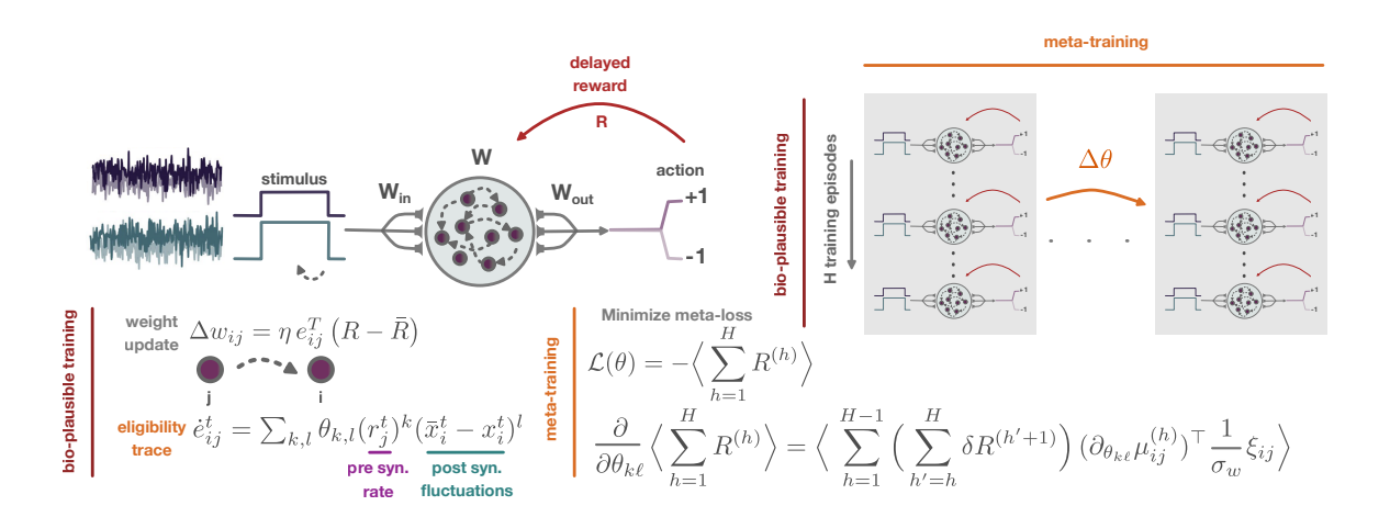
Figure 1: Outline of the proposed meta-learning framework.

plasticity rules capable of supporting structured credit assignment from delayed feedback remains vastly underexplored.

Backpropagation through time (BPTT), the standard approach for training recurrent neural networks (RNNs), is biologically implausible since it requires symmetric forward and backward connections and non-local information (Lillicrap et al., 2016; Guerguiev et al., 2017). Although recent work has reformulated BPTT into more biologically plausible variants using random feedback (Lillicrap et al., 2016; Murray, 2019), truncated approximations, or by learning feedback pathways (Lindsey and Litwin-Kumar, 2020; Shervani-Tabar and Rosenbaum, 2023), these methods require continuous error signals to refine recurrent connections.

Here, we adopt a bottom-up approach: instead of imposing hand-designed synaptic rules, we discover biologically plausible plasticity rules that support learning through delayed reinforcement signals via meta-optimisation (Schmidhuber et al., 1996). Building on recent work (Confavreux et al., 2023), we parameterise plasticity rules as functions of local signals (presynaptic activity, postsynaptic activity, and synapse size) and meta-learn their parameters within a second reinforcement learning loop. With that, our ongoing work tackles the following questions:

• Which local learning rules can implement structured credit assignment under biological constraints?
• Do different plasticity rules give rise to different representations and/or dynamics?

Here we demonstrate that different forms of plasticity naturally lead to qualitatively different learning trajectories and internal representations, akin to their gradient-based counterparts trained with different learning rules.

2. Method

Network dynamics. We consider recurrent neural networks of firing rate neurons coupled through a synaptic matrix $\mathbf{W} \in \mathcal{R}^{N \times N}$ (Sompolinsky et al., 1988; Barak, 2017), with additional input and output matrices $\mathbf{W}_{\text{in}} \in \mathcal{R}^{N \times N_{\text{in}}}$ and $\mathbf{W}_{\text{out}} \in \mathcal{R}^{N_{\text{out}} \times N}$ that route task-relevant input into the recurrent circuit and read out network activation to generate task-specific outputs (actions). The equations governing the network dynamics are

$$\frac{d\mathbf{x}^{t}}{dt} = -\mathbf{x}^{t} + \mathbf{W}\phi(\mathbf{x}^{t}) + \mathbf{W}_{\text{in}}\mathbf{u}^{t}, \qquad \mathbf{r}^{t} = \phi(\mathbf{x}^{t}) \dot{=} \tanh(\mathbf{x}^{t}), \tag{1}$$

where $\mathbf{x}^t \in \mathcal{R}^N$ is the vector of pre-activations (or input currents) to each neuron in the network, $\phi(\cdot): \mathcal{R}^N \to \mathcal{R}^N$ denotes the single-neuron transfer functions, $\mathbf{r}^t \in \mathcal{R}^N$ is the vector of instantaneous firing rates, $\mathbf{u}^t$ stands for the activity of the $N_{\rm in}$ input neurons. In the terms above, the $\cdot^t$ superscript indicates time dependence. Network outputs $\mathbf{z}^t$ are obtained from linear read-out neurons as $\mathbf{z}^t = \mathbf{W}_{\rm out} \mathbf{r}^t$ .

Sparse feedback and parametrized learning rules. We consider networks that learn cognitive tasks using biologically plausible local learning rules, guided by sparse reinforcement signals R provided only at the end of each training episode. Each synapse between a pre-synaptic unit j and a post-synaptic unit i maintains an eligibility trace $e_{ij}$ (Izhikevich, 2007), which integrates the history of (co-)activation during the episode. We define the evolution of eligibility traces with differential equations of the form

$$\frac{\mathrm{d}e_{ij}^t}{\mathrm{d}t} = \mathcal{H}_{\theta}(r_j^t, x_i^t) - \frac{e_{ij}^t}{\tau_e} = \sum_{0 \le k: \ell \le d:} \theta_{k,\ell} \left(r_j^t\right)^k \left(\bar{x}_i - x_i^t\right)^\ell - \frac{e_{ij}^t}{\tau_e},\tag{2}$$

where $\tau_e$ is a decay time-scale, $\bar{x}_i$ is a running average of the pre-activation of neuron i, and $\theta_{k,\ell} \in \mathcal{R}$ are learnable coefficients. In contrast to eligibility traces based solely on first-order correlations (Gerstner et al., 2018), we use here a polynomial expression that captures richer interactions between pre- and post-synaptic activity. Each coefficient $\theta_{k,\ell}$ can be construed as a term-specific learning rate, which may be positive (Hebbian), negative (anti-Hebbian), or zero. In our experiments, we set d=5.

The recurrent weight matrix $\mathbf{W}$ gets updated at the end of each training episode according to a reward-modulated learning rule

$$\pi_{\Theta}\left(\mathbf{\Delta}\mathbf{W}^{(h)} \mid \mathbf{\Theta}\right) = \mathcal{M}\mathcal{N}\left(\boldsymbol{\mu}_{\mathbf{\Theta}}^{(h)}, \, \sigma_{w}^{2} \, \mathbf{I}_{N}, \mathbf{I}_{N}\right) \quad \text{with} \quad [\boldsymbol{\mu}_{\mathbf{\Theta}}^{(h)}]_{ij} = \eta \, e_{ij}^{T_{h}} \, \left(R^{(h)} - \bar{R}^{(h)}\right), \tag{3}$$

where with $\mathcal{MN}(\mu, \Sigma, \mathbf{V})$ we denote the matrix normal distribution with mean $\mu \in \mathbb{R}^{N \times N}$ , and $\Sigma$ and $\mathbf{V}$ the positive semi-definite matrices are the row- and column-variance, while superscript h indicates episode index, $\eta$ denotes the learning rate, $e_{ij}^{T_s}$ stands for the eligibility trace accumulated till the end of the h-th episode $T_h$ , while R, R stand for the obtained and the expected reward. Here, we model reward expectations for each type of trial independently as a running average of past rewards for this trial type (Miconi, 2017). This update rule enables credit assignment through the interaction between synaptic eligibility and trial-specific reward prediction error, consistent with neo-Hebbian three-factor learning rules hypothesized to operate in biological circuits (Gerstner et al., 2018).

Meta-learning plasticity rules. While previous work has relied on hand-crafted eligibility trace dynamics and synaptic update rules to train recurrent neural networks with sparse feedback (Miconi, 2017), we instead adopt a meta-learning approach to learn the parameters of the plasticity rules. Our framework consists of two nested training loops: (i) an inner loop in which the recurrent network is trained over several episodes using local learning rules and sparse reinforcement signals provided at the end of each episode (bio-plausible training), as described above; and (ii) an outer loop that optimizes the plasticity meta-parameters $\Theta = \{\{\theta_{k,\ell}\}_{k,\ell=0}^5\}$ via gradient descent using tangent-propagation through learning (forward-mode differentiation through learning) on a meta-loss computed over H training episodes (trials) (meta-training). This approach allows the learning rules themselves to be adapted to the task, rather than be fixed a priori.

Tangent-propagation through learning. Our goal is to optimise the learning rule parameters $\Theta$ to maximise task performance, quantified as the expected cumulative reward $\langle \sum_h R \rangle$ obtained after a fixed number of learning episodes. However, the reward R depends on the network's output, which is determined by synaptic weights $\mathcal{W} = \{\mathbf{W}_{in}, \mathbf{W}, \mathbf{W}_{out}\}$ , with $\mathbf{W}$ evolving under the update rule (Eq.3). Since weights depend on eligibility traces $e_{ij}$ , themselves parameterised by $\Theta$ , the reward depends on the plasticity parameters through $\mathcal{W}$ and $\Theta$ . Directly computing $\nabla_{\Theta}\langle \sum_h R \rangle$ by backpropagating through the learning dynamics is computationally prohibitive since learning requires several hundreds of trials (Lindsey and Litwin-Kumar, 2020). We therefore, here, adopt a REINFORCE-inspired estimator (Williams, 1992), which involves computing the gradient of an expected value by observing outcomes (the rewards) and scaling a measure of what elicited that outcome (the weight updates) with the associated reward. Thus, we approximate the gradient of the expected reward by

$$\nabla_{\Theta} \langle \sum_{h} R^{(h)} \rangle \approx \langle \sum_{h} \sum_{h'=h+1}^{H} R^{(h')} \nabla_{\Theta} \log \pi (\mathbf{\Delta} \mathbf{W}^{(h)} \mid \mathbf{\Theta}) \rangle \approx \langle \sum_{h} \sum_{h'=h+1}^{H} (R^{(h')} - \bar{R}^{(h')}) \nabla_{\Theta} \log \pi (\mathbf{\Delta} \mathbf{W}^{(h)} \mid \mathbf{\Theta}) \rangle, \tag{4}$$

where $\bar{R}$ stands for the baseline reward, and thus $(R-\bar{R})$ denotes the reward prediction error. Introducing the expression of the plasticity rule, we have in a component-wise formulation for each dimensional component of the plasticity parameters $\Theta$

$$\frac{\partial}{\partial \theta_{k,\ell}} \left\langle \sum_{h=1}^{H-1} R^{(h)} \right\rangle = \left\langle \sum_{h=1}^{H-1} \left( \sum_{h'=h}^{H-1} \delta R^{(h'+1)} \right) \frac{1}{\sigma_w^2} \sum_{i=1}^{N} \sum_{j=1}^{N} \left( \Delta w_{ij}^{(h)} - \mu_{ij}^{(h)} \right) \frac{\partial \mu_{ij}^{(h)}}{\partial \theta_{k,\ell}} \right\rangle_S, \quad (5)$$

where the expectation $\langle \cdot \rangle_S$ is considered over independent sessions S. This requires the computation of the sensitivity of the mean weight update wrt to the plasticity parameters $\frac{\partial \mu_{ij}^{(h)}}{\partial \theta_{kl}}$ over training. To that end, we propagate the gradients of the within-trial pre-activations $\mathbf{x}^t$ , $\mathbf{\chi}_{k,\ell}^t \in \mathcal{R}^N$ (state tangent), the pre-activation trace $\bar{\mathbf{x}}^t$ , $\psi_{k,\ell}^t \in \mathcal{R}^N$ (trace tangent), and of the eligibility traces of each synaptic pair ij, $e_{ij}^t$ , $[\mathbf{z}_{k,\ell}^t]_{ij}$ (eligibility tangent), as well as inter-trial sensitivities of weight matrices (weight matrix tangent), $\mathbf{U}_{k,\ell}^{(h)}$ (c.f. Appendix Sec. C).

References

• Malbor Asllani and Timoteo Carletti. Topological resilience in non-normal networked systems. Physical Review E, 97(4):042302, 2018.
• Malbor Asllani, Renaud Lambiotte, and Timoteo Carletti. Structure and dynamical behavior of non-normal networks. Science Advances, 4(12):eaau9403, 2018.
• Craig H Bailey and Eric R Kandel. Structural changes accompanying memory storage. Annual Review of Physiology, 1993.
• Omri Barak. Recurrent neural networks as versatile tools of neuroscience research. Current Opinion in Neurobiology, 46:1–6, 2017.
• Sam E Benezra, Kripa B Patel, Citlali P´erez Campos, Elizabeth MC Hillman, and Randy M Bruno. Learning enhances behaviorally relevant representations in apical dendrites. Elife, 13:RP98349, 2024.
• Guo-qiang Bi and Mu-ming Poo. Synaptic modifications in cultured hippocampal neurons: dependence on spike timing, synaptic strength, and postsynaptic cell type. Journal of Neuroscience, 18(24):10464–10472, 1998.
• Brian Blais, Nathan Intrator, Harel Shouval, and Leon Cooper. Receptive field formation in natural scene environments: comparison of single cell learning rules. Advances in Neural Information Processing Systems, 10, 1997.
• Carlos SN Brito and Wulfram Gerstner. Nonlinear hebbian learning as a unifying principle in receptive field formation. PLoS computational biology, 12(9):e1005070, 2016.
• Georgia Christodoulou, Tim P Vogels, and Everton J Agnes. Regimes and mechanisms of transient amplification in abstract and biological neural networks. PLoS Computational Biology, 18(8):e1010365, 2022.
• Basile Confavreux, Poornima Ramesh, Pedro J Goncalves, Jakob H Macke, and Tim Vogels. Meta-learning families of plasticity rules in recurrent spiking networks using simulationbased inference. Advances in Neural Information Processing Systems, 36:13545–13558, 2023.
• Wulfram Gerstner, Marco Lehmann, Vasiliki Liakoni, Dane Corneil, and Johanni Brea. Eligibility traces and plasticity on behavioral time scales: experimental support of neohebbian three-factor learning rules. Frontiers in Neural Circuits, 12:53, 2018.
• Michael Graupner and Nicolas Brunel. Calcium-based plasticity model explains sensitivity of synaptic changes to spike pattern, rate, and dendritic location. Proceedings of the National Academy of Sciences, 109(10):3991–3996, 2012.
• Jordan Guerguiev, Timothy P Lillicrap, and Blake A Richards. Towards deep learning with segregated dendrites. Elife, 6:e22901, 2017.

Maoutsa

• Robert G¨utig, Ranit Aharonov, Stefan Rotter, and Haim Sompolinsky. Learning input correlations through nonlinear temporally asymmetric hebbian plasticity. Journal of Neuroscience, 23(9):3697–3714, 2003.
• John J Hopfield. Neural networks and physical systems with emergent collective computational abilities. Proceedings of the National Academy of Sciences, 79(8):2554–2558, 1982.
• Eugene M Izhikevich. Solving the distal reward problem through linkage of stdp and dopamine signaling. Cerebral Cortex, 17(10):2443–2452, 2007.
• Lukasz Ku´smierz, Takuya Isomura, and Taro Toyoizumi. Learning with three factors: modulating hebbian plasticity with errors. Current Opinion in Neurobiology, 46:170–177, 2017.
• C Charles Law and Leon N Cooper. Formation of receptive fields in realistic visual environments according to the bienenstock, cooper, and munro (bcm) theory. Proceedings of the National Academy of Sciences, 91(16):7797–7801, 1994.
• Christiane Lemieux. Control variates. Wiley StatsRef: Statistics Reference Online, pages 1–8, 2014.
• Timothy P Lillicrap, Daniel Cownden, Douglas B Tweed, and Colin J Akerman. Random synaptic feedback weights support error backpropagation for deep learning. Nature Communications, 7(1):13276, 2016.
• Jack Lindsey and Ashok Litwin-Kumar. Learning to learn with feedback and local plasticity. Advances in Neural Information Processing Systems, 33:21213–21223, 2020.
• Stephen J Martin, Paul D Grimwood, and Richard GM Morris. Synaptic plasticity and memory: an evaluation of the hypothesis. Annual Review of Neuroscience, 23(1):649– 711, 2000.
• Mark Mayford, Steven A Siegelbaum, and Eric R Kandel. Synapses and memory storage. Cold Spring Harbor perspectives in biology, 4(6):a005751, 2012.
• Thomas Miconi. Biologically plausible learning in recurrent neural networks reproduces neural dynamics observed during cognitive tasks. Elife, 6:e20899, 2017.
• Thomas Miconi, Kenneth Stanley, and Jeff Clune. Differentiable plasticity: training plastic neural networks with backpropagation. In International Conference on Machine Learning, pages 3559–3568. PMLR, 2018.
• Brendan K Murphy and Kenneth D Miller. Balanced amplification: a new mechanism of selective amplification of neural activity patterns. Neuron, 61(4):635–648, 2009.
• James M Murray. Local online learning in recurrent networks with random feedback. Elife, 8:e43299, 2019.
• Victor Pedrosa and Claudia Clopath. Voltage-based inhibitory synaptic plasticity: network regulation, diversity, and flexibility. bioRxiv, pages 2020–12, 2020.

Juergen Schmidhuber, Jieyu Zhao, and MA Wiering. Simple principles of metalearning. Technical report IDSIA, 69:1–23, 1996.

Navid Shervani-Tabar and Robert Rosenbaum. Meta-learning biologically plausible plasticity rules with random feedback pathways. Nature Communications, 14(1):1805, 2023.

Per Jesper Sj¨ostr¨om, Gina G Turrigiano, and Sacha B Nelson. Rate, timing, and cooperativity jointly determine cortical synaptic plasticity. Neuron, 32(6):1149–1164, 2001.

Haim Sompolinsky, Andrea Crisanti, and Hans-Jurgen Sommers. Chaos in random neural networks. Physical Review Letters, 61(3):259, 1988.

Baram Sosis and Jonathan E Rubin. Distinct dopaminergic spike-timing-dependent plasticity rules are suited to different functional roles. bioRxiv, 2024.

Ronald J Williams. Simple statistical gradient-following algorithms for connectionist reinforcement learning. Machine Learning, 8(3-4):229–256, 1992.

Appendix A. Plasticity gradient with REINFORCE approximation

Following the REINFORCE estimator (Williams, 1992), we approximate the gradient of the expected reward by

$$\nabla_{\theta} \langle R \rangle = \langle (R - \bar{R}) \nabla_{\theta} \log \pi (\mathbf{\Delta W} \mid \theta) \rangle. \tag{6}$$

This results from applying the log-derivative trick on the expectation of Eq. 6

$$\begin{split} \nabla_{\theta} \langle R \rangle &= \nabla_{\theta} \int \pi(\Delta \mathbf{W} \mid \theta) \, R \, \mathrm{d} \Delta \mathbf{W} \\ &= \int \nabla_{\theta} \pi(\Delta \mathbf{W} \mid \theta) \, R \, \mathrm{d} \Delta \mathbf{W} \qquad \text{(Leibniz integral rule)} \\ &= \int \pi(\Delta \mathbf{W} \mid \theta) \, \frac{\nabla_{\theta} \pi(\Delta \mathbf{W} \mid \theta)}{\pi(\Delta \mathbf{W} \mid \theta)} \, R \, \mathrm{d} \Delta \mathbf{W} \\ &= \int \pi(\Delta \mathbf{W} \mid \theta) \, \nabla_{\theta} \log \pi(\Delta \mathbf{W} \mid \theta) \, R \, \mathrm{d} \Delta \mathbf{W} \qquad \text{(log-derivative trick)} \\ &= \langle R \, \nabla_{\theta} \log \pi(\Delta \mathbf{W} \mid \theta) \rangle_{\pi} \\ &\approx \left\langle \begin{array}{c} (R - \bar{R}) \\ \text{reward prediction} \end{array} \right. \nabla_{\theta} \log \pi(\Delta \mathbf{W} \mid \theta) \right\rangle. \end{split}$$

In the last expression we have introduced the baseline reward R¯ as a control variate (Lemieux, 2014) commonly used for variance reduction of the expectation. This heuristic uses the reward prediction error δR = R − R¯ as a scaling factor for the direction of the update. This approximation assumes that R is a smooth functional of W and that changes in θ affect R primarily through their effect on the connectivity W.

Appendix B. Analysis of dynamics for each network

Numerical solver. We located fixed points by solving for G(x) = 0 with

$$\mathbf{G}(\mathbf{x}) = \mathbf{x} - \mathbf{W}\phi(\mathbf{x}) - \mathbf{W}_{\text{in}}\mathbf{u},$$

using a damped Newton method. To avoid identifying duplicate fixed points, we initialized from 200 random initial conditions and discarded solutions within a distance of $\gamma \leq 1e-5$ of one another. This resulted in a set of unique fixed points per input condition.

Jacobian definition. We linearized the dynamics at the vicinity of each fixed point $\mathbf{x}^*$ . The Jacobian is defined as

$$\mathbf{J}(\mathbf{x}^*) = -\mathbf{I}_N + \mathbf{W}\operatorname{diag}(1 - \phi^2(\mathbf{x}^*)), \qquad (7)$$

and governs the local flow $\dot{\delta \mathbf{x}} = \mathbf{J} \, \delta \mathbf{x}$ .

Stability criteria. A fixed point is linearly stable if $\max \Re(\lambda(\mathbf{J})) < 0$ .

Eigenmode analysis. From the eigenvalues and eigenvectors of J, we extracted several diagnostics:

• Time constants and frequencies: Each mode with eigenvalue $\lambda = \beta + i\omega$ corresponds to a decay time $-\frac{1}{\beta}$ (if $\beta < 0$ ) and an oscillation frequency $\omega/2\pi$ .
• Non-normality: Since the Jacobian eigenvectors are not orthogonal, small perturbations can have large transient effects even if all eigenvalue real parts are negative. Thus, we quantified the departure from normality with the Henrici index $\|\mathbf{J}\|_F^2 \sum_i |\lambda_i|^2$ (Murphy and Miller, 2009; Asllani et al., 2018), which is indicative of transient amplification, where $\|\cdot\|_F$ stands for the Frobenius norm.
• Transient gain: We measured $\max_t \|e^{\mathbf{J}t}\|_2$ on a grid of times t (Christodoulou et al., 2022; Asllani and Carletti, 2018), capturing the degree of short-term amplification even when the dynamics are asymptotically stable.
• Readout alignment: We computed the overlap of the corresponding readout vector $\mathbf{w}_{\text{out}}$ with the eigenvectors of $\mathbf{J}$ , to identify which eigenmodes directly influence network output. For each mode i, we characterise the alignment by

$$a_i = \|\langle \mathbf{w}_{\text{out}}, \mathbf{v}_i \rangle\|, \tag{8} $$

where $\mathbf{v}_i$ are the normalized right eigenvectors of J. Large $a_i$ values indicate that the corresponding i-th mode contributes strongly to the output. In strongly non-normal systems we additionally verified projections using left–right biorthogonal eigenvectors.

• Susceptibility: We computed the linear response $\mathbf{p} = (-\mathbf{J})^{-1}\mathbf{W}_{in}$ , quantifying the steady-state sensitivity of each neuron to perturbations in the input.

Appendix C. Tangent-propagation through learning

Tangent-propagation through single trial time. To be able to compute the gradient of the weight updates with respect to the plasticity parameters, we propagate the gradients of the within-trial pre-activations $\mathbf{x}^t$ , $\chi_{k,\ell}^t \in \mathcal{R}^N$ (state tangent), the pre-activation trace $\bar{\mathbf{x}}^t$ , $\psi_{k,\ell}^t \in \mathcal{R}^N$ (trace tangent), and of the eligibility traces of each synaptic pair ij, $e_{ij}^t$ , $[\mathbf{z}_{k,\ell}^t]_{ij}$ (eligibility tangent). Thus we define the following within-trial tangents (sensitivities) with respect to the plasticity parameter $\theta_{k,\ell}$

$$\chi_{k,\ell}^t = \frac{\partial \mathbf{x}^t}{\partial \theta_{k,\ell}}, \qquad \psi_{k,\ell}^t = \frac{\partial \bar{\mathbf{x}}^t}{\partial \theta_{k,\ell}}, \qquad \mathbf{z}_{k,\ell}^t = \frac{\partial \mathbf{e}^t}{\partial \theta_{k,\ell}}. \tag{9} $$

We assume that the reward and baseline reward R and $\bar{R}$ are not directly related to the plasticity parameters $\theta_{k,\ell}$ , and thus we treat these variables and the reward prediction error as $\theta$ -independent.

For convenience we define $\alpha = \mathrm{d}t/\tau$ , and denote the derivative of the single neuron activation function with $\mathrm{d}\phi(x) = \phi'(x)\,\mathrm{d}x$ . The forward equations for these sensitivity parameters are

$$\chi_{k,\ell}^{t+1} = \chi_{k,\ell}^{t} + \alpha \left( -\chi_{k,\ell}^{t} + \mathbf{W}^{(h)} \left( \operatorname{diag}(\phi'(\mathbf{x}^{t})) \cdot \chi_{k,\ell}^{t} \right) + \mathbf{U}_{k,\ell}^{(h)} \mathbf{r}^{t} \right) \psi_{k,\ell}^{t+1} = \alpha_{x} \psi_{k,\ell}^{t} + (1 - \alpha_{x}) \chi_{k,\ell}^{t+1}, \mathbf{z}_{k,\ell}^{t+1} = \mathbf{z}_{k,\ell}^{t} + \operatorname{d}t \left( \Delta \mathbf{x}^{t} \right)^{\ell} \otimes \left( \mathbf{r}^{t} \right)^{k} + \operatorname{d}t \sum_{\kappa,\lambda} \left[ \theta_{\kappa,\lambda} \lambda \left( \Delta \mathbf{x}^{t} \right)^{\lambda-1} (\psi_{k,\ell}^{t} - \chi_{k,\ell}^{t+1}) \otimes \left( \mathbf{r}^{t} \right)^{\kappa} + \theta_{\kappa,\lambda} \left( \Delta \mathbf{x}^{t} \right)^{\lambda} \otimes \kappa \left( \mathbf{r}^{t} \right)^{\kappa-1} \left( \operatorname{diag}(\phi'(\mathbf{x}^{t})) \cdot \chi_{k,\ell}^{t} \right) \right],$$

where $diag(\mathbf{y})$ denotes the matrix with $\mathbf{y}$ in the main diagonal, $\otimes$ denotes the outer product, while

$$\mathbf{U}_{k,\ell}^{(h)} \doteq \frac{\partial \mathbf{W}^{(h)}}{\partial \theta_{k,\ell}} \tag{11}$$

stands for the inter-trial weight matrix tangent. The initial conditions for the three sensitivity parameters are zero at the beginning of each trial $\chi_{k,\ell}^0 = \mathbf{0}$ , $\psi_{k,\ell}^0 = \mathbf{0}$ , and $\mathbf{z}_{k,\ell}^0 = \mathbf{0}$ .

At the end of each trial h we have

$$\frac{\partial \boldsymbol{\mu}^{(h)}}{\partial \theta_{k,\ell}} = \eta \, \delta R^{(h)} \, \mathbf{z}_{k,\ell}^{T_h} \,. \tag{12}$$

Propagating sensitivities through-learning (across trials). The derivative of the weights of trial h + 1 w.r.t. $\theta_{k,\ell}$ accumulates the across trial sensitivities

$$\mathbf{U}_{k,\ell}^{(h+1)} = \mathbf{U}_{k,\ell}^{(h)} + \frac{\partial \boldsymbol{\mu}^{(h)}}{\partial \theta_{k,\ell}}, \quad \text{with } \mathbf{U}_{k,\ell}^{(0)} = 0. \tag{13} $$

This sensitivity $\mathbf{U}_{k,\ell}^{(h)}$ couples back into the state tangent through the $\mathbf{U}_{k,\ell}^{(h)}\mathbf{r}^t$ term, which captures how $\theta_{k,\ell}$ affects later trials through the modified weights of earlier trials.

C.1. Validation of weight updates gradients wrt plasticity parameters

To validate the gradients wrt plasticity parameters obtained through forward mode differentiation, we compare both single-trial and multi-trial gradients (for H=500 trials) obtained with finite differences (FD) to those computed through forward mode differentiation (FM). To avoid observing discrepancies between the two versions of the gradients, we employ the same noise and environment inputs in all simulations. For this experiment we considered only $\theta_{3,3}=1$ nonzero, while all other entries of $\Theta$ were zero. For the finite difference calculation, we run the training with $\theta+\epsilon$ and $\theta-\epsilon$ for $\epsilon=10^{-4}$ and approximate the gradient of the weight update with respect to the plasticity parameter as

$$\frac{\mathrm{d}\Delta\mathbf{W}}{\mathrm{d}\theta_{k,\ell}} \approx \frac{\Delta\mathbf{W}^{+}\left(\theta_{k,\ell} + \varepsilon\right) - \Delta\mathbf{W}^{-}\left(\theta_{k,\ell} - \varepsilon\right)}{2\varepsilon}. \tag{14} $$

The resulting two versions of the gradients are in very close agreement throughout all 500 trials (Fig. 2).

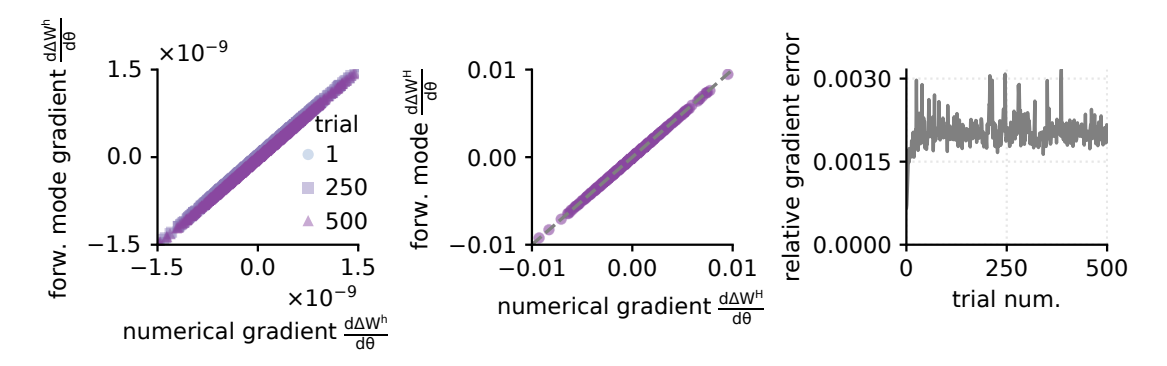
Figure 2: Validation of forward-mode gradient (FM) computation for the weight update wrt plasticity parameters $\theta$ against numerical gradients (FD). a. Comparison of numerical gradient for per-trial weight update $\Delta \mathbf{W}^{(h)}$ wrt plasticity parameter $\theta_{3,3}$ against the gradient obtained through forward mode differentiation for trials 1,250,500 . b. Comparison of cumulative gradient computed over 500 trials for the weight update wrt plasticity parameters obtained numerically and through forward mode differentiation. The forward-mode differentiation provides an exact estimation of the plasticity update gradients. c. Relative gradient error per trial computed as $\|\frac{\mathbf{d}\Delta \mathbf{W}}{\mathbf{d}\theta}^{FM} - \frac{\mathbf{d}\Delta \mathbf{W}}{\mathbf{d}\theta}^{FD}\|/\|\frac{\mathbf{d}\Delta \mathbf{W}}{\mathbf{d}\theta}^{FD}\|$ .