title: Scaling_machine_learning_and_genetic_neu
source_pdf: /home/lzr/code/thesis-reading/Neuroevolution/Chapter 3/Scaling_machine_learning_and_genetic_neu.pdf
Scaling, Machine Learning, and Genetic Neural Nets
ERIC MJOLSNESS*
Department of Computer Science, Yale University, New Haven, Connecticut 06520
DAVID H. SHARP†
Theoretical Division, Los Alamos National Laboratory, Los Alamos, New Mexico 87545
AND BRADLEY K. ALPERT*
Department of Computer Science, Yale University, New Haven, Connecticut 06520
We consider neural nets whose connections are defined by growth rules taking the form of recursion relations. These are called genetic neural nets. Learning in these nets is achieved by simulated annealing optimization of the net over the space of recursion relation parameters. The method is tested on a previously defined continuous coding problem. Results of control experiments are presented so that the success of the method can be judged. Genetic neural nets implement the ideas of scaling and parsimony, features which allow generalization in machine learning. © 1989 Academic Press, Inc.
1. INTRODUCTION
Can a machine generalize as it learns? The question must be properly framed before the answer is valuable. If the problem of machine learning is posed as one of neural net optimization [5, 19], a precise scientific context is established in which to explore questions such as generalization.
A synthetic neural net is a particular kind of circuit parameterized by real-valued connection strengths between circuit elements called "neurons." Machine learning can be posed as the problem of optimizing some real-valued function of a network over its parameter space. Such optimization often involves measuring a network's performance on a fixed set of inputs called the training set. If the network then
*Work supported in part by ONR Grant N00014-86-K-0310.
†Work supported by DOE.
performs acceptably on a predictable set of inputs much larger than the training set, it has generalized.
What enables a neural net to generalize? We focus on the properties of scaling and parsimony.
The information in a neural net is contained in its pattern of connection strengths. Parsimony in a network means that this information is expressed as succinctly as possible without compromising performance. It aids generalization by reducing the size of the search space, and therefore the number of nets which coincidentally do well on the training set but do not generalize.
The idea of scaling is to solve small problems, where a large fraction of the possible inputs can be sampled as the network learns, and to use the results to automatically generate nets which solve bigger problems. Scaling may also be thought of as extrapolation and hence generalization along a scale axis. This kind of generalization is of critical importance for all considerations of cost in neural net computing and learning.
To construct neural nets which exhibit scaling and parsimony requires a fundamental shift from the optimization of neural nets to the optimization of relatively simple growth rules for constructing nets. As a model for what is intended, recall that genetically prescribed growth rules for biological neural nets are far more concise than the synapses they determine. For example, the human genome has been estimated to contain 30,000 genes with an average of 2,000 base pairs each [12], for a total of roughly 108 base pairs; this is clearly insufficient to independently specify the 1015 synapses [9] in the human brain. Instead the genes probably specify rules for network growth, as well as rules by which individual synapses can learn from experience.
The growth rules introduced in this paper are specified in terms of underlying "genetic" information, which is taken to consist of a fixed number of real-valued coefficients in a recursion relation defining a family of successively larger neural nets. Even though our growth rules are not directly modelled after any biological system, we summarize the fundamental shift to the optimization of growth rules by describing the resulting artificial circuits as "genetic neural nets."
Since any growth rule can generate nets of unbounded size, a genetic neural net will generally have many more connection strengths than there are coefficients in its recursion relation. Then the net is parsimonious. Indeed, the potential information content of the wiring in any neural net is proportional to its number of connections, whereas the actual information content of the wiring in a genetic neural net is at most the number of coefficients in the recursion relation that generated it. (We assume that the number of bits which can be stored in each connection strength or recursion coefficient is small.) Parsimonious nets are also called "structured" nets, and
learning rules for unstructured nets, or mixtures of the two types of nets, are outside the scope of this paper.
From a programmer's or circuit designer's point of view, genetic neural nets involve two fundamental principles: "divide-and-conquer" and "super position". The main idea of the divide-and-conquer strategy is to break up a big problem into small pieces, each of which can be solved by the same method, and then to combine the solutions. We mention the merge-sort algorithm, fast Fourier transform and Karp's algorithm for the Traveling Salesman Problem in the Euclidean plane as examples of algorithms which use this strategy. Superposition is a property which applies to the connection strength between pairs of circuit elements or neurons. The set of all such numbers in one net may be considered as a matrix, called the connection matrix, indexed by pairs of neurons. In the context of neural networks, it has been found that a network formed by addition or "superposition" of the connection matrices of simpler networks is frequently able to perform a combination of the simpler networks' tasks [7, 8]. These ideas are combined in Section 2 to derive a generic, or problem-independent, recursion relation for connection matrices. An infinite family of successively larger connection matrices, called a template, is specified by each such recursion relation.
Our strategy for machine learning with scaling and parsimony consists of the following steps: (1) A recursion relation generates a family of related connection matrices of increasing size. Families of connection matrices form a search space. This space is parameterized using the coefficients of the corresponding recursion relations. (Section 2.1). (2) A sequence of learning tasks of increasing size is specified by choosing a task functional of the connection matrices. Learning is achieved as this functional is minimized over the coefficients in the recursion relation (Section 2.2). (3) The task functional is combined with a parsimony constraint on the allowed recursion relations, which requires that the number or information content of the coefficients be small, to produce a global optimization problem, which defines a dynamics on the space of recursion relations. (4) The optimization problem so defined is infinite, and for practical purposes must be replaced by a finite version. This is done by optimizing, or training, the recursion relation on a finite number of small tasks and using the results to perform larger tasks, without further training. In this way our procedure obtains learning with generalization.
This circle of ideas has been tested by means of numerical simulation on a coding problem (Section 3). Control experiments are presented so that the success of our method can be judged. Suggestions for extensions of this work are contained in a concluding section. A preliminary account of some of the ideas presented here has appeared previously [14, 15].
2. GENETIC NEURAL NETWORKS
This section contains three parts; the first presents our method for the recursive description of connection matrices, the second outlines the method for optimizing them, and the third compares the method with related work.
2.1. The Recursive Description of Connection Matrices
The recursive description of connection matrices requires the following basic ingredients: (1) a method for indexing circuit elements or "neurons" by specifying their position in a binary tree (a lineage, tree) of circuit elements. (2) A family of such trees parameterized by an integer specifying the problem size. (3) Recursion relations. Lineage trees are related to connection matrices in that a given element of a connection matrix is indexed by an ordered pair of nodes in a lineage tree. Connection matrices as well as lineage trees of different sizes are related by recursion relations. (4) Two sets of parameters in the recursion relations. Decomposition matrices define the relationship between connection matrices in successive generations of a family. A set of basis values complete the determination of the connection matrix when a recursion relation is terminated after a finite number of steps. The values of all of these parameters are obtained by means of the optimization procedure discussed in Section 2.2.
To bring these ideas into focus, we begin with an example. Consider the following matrix which represents the connections of a simple 1-dimensional chain of neurons
$$\begin{pmatrix} 0 & 1 & 0 & 0 & 0 & 0 & 0 \\ 0 & 0 & 1 & 0 & 0 & 0 & 0 \\ 0 & 0 & 0 & 1 & 0 & 0 & 0 & 0 \\ \hline 0 & 0 & 0 & 0 & 1 & 0 & 0 & 0 \\ 0 & 0 & 0 & 0 & 0 & 1 & 0 & 0 \\ 0 & 0 & 0 & 0 & 0 & 0 & 1 & 0 \\ 0 & 0 & 0 & 0 & 0 & 0 & 0 & 1 \\ 0 & 0 & 0 & 0 & 0 & 0 & 0 & 0 \end{pmatrix} \tag{1}$$
Here a 1 in position (i, j) denotes a connection from neuron i to neuron j. Thus the matrix represents a chain of neurons in which the first is connected
to the second, the second to the third, etc. The matrix may be viewed as four quadrants such that the upper-left and lower-right quadrants resemble the entire matrix, the upper-right contains a single 1 in its lower-left corner, and the lower-left quadrant is all zeroes.
We introduce an infinite family of matrices of the form (1), $\tau_1(n)$ , and refer to the family $\tau_1$ as a template. The upper right quadrant of (1) is a member of a second family $\tau_2$ . The pattern present in the families of matrices $\tau_1$ and $\tau_2$ can be expressed recursively;
$$\tau_{1}(n+1) = \begin{pmatrix} \tau_{1}(n) & \tau_{2}(n) \\ 0 & \tau_{1}(n) \end{pmatrix},$$
$$\tau_{2}(n+1) = \begin{pmatrix} 0 & 0 \\ \tau_{2}(n) & 0 \end{pmatrix} \tag{2} $$
The basis values $\tau_1(0)$ and $\tau_2(0)$ are not determined by (2); they must be supplied separately. In this example, $\tau_1(0) = 0$ and $\tau_2(0) = 1$ . To expand the recursion relation (2), each of the four quadrants of a template is expanded recursively unless n = 1, in which case the relevant basis value is substituted for that quadrant. This notion of a template may be generalized somewhat so that each quadrant of a template is expressed as a linear combination of other templates with real-number weights.
In the Appendix we provide similar recursive descriptions for connection matrices corresponding to 2- and 3-dimensional grids of neurons.
The $\tau_a(n)$ notation enables us to represent entire connection matrices recursively. We need, however, to produce recursion equations for individual matrix entries (the connection weights). To do so, we develop a method of addressing, or indexing, each entry through the idea of a lineage tree of neurons. Imagine the recursive iteration of Eq. (2) run backwards, from large to small matrices. At each stage, the set of neurons labeling the rows or columns is divided into two groups labeled "left" and "right." A given neuron can be uniquely indexed by specifying a sequence of binary decisions as to whether it belongs to the "left" or "right" group at each stage. The sequence of divisions of neurons into smaller groups defines a binary tree, the lineage tree, whose terminal nodes are the neurons. Each neuron is now indexed by a string of 0's (left) and 1's (right) defining a path through the tree. This string defines the "address" of the neuron and is denoted by $i_1$ , . . . , $i_n$ . A generic element of this string will be denoted p or q. Figure 1 shows a lineage tree of neurons and their addresses.
Let us rewrite Eq. (2) using the lineage tree indexing of "neurons." An arbitrary element of a connection matrix is now addressed by an ordered
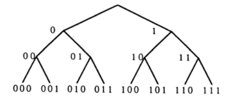
FIG. 1. Lineage tree of neurons and their addresses.
pair of neuron addresses. For a connection matrix $\tau_a(n)$ , the entry denoting the connection strength from the neuron with address $i_1 \ldots i_n$ to the neuron with address $j_1 \ldots j_n$ is $T_{i_1 \ldots i_n, j_1 \ldots j_n}$ . In this notation,
$$\tau_1(n) = \begin{pmatrix} \tau_1(n-1) & \tau_2(n-1) \\ 0 & \tau_1(n-1) \end{pmatrix}$$
represents $2^{2n}$ equations, four of which are
$$T_{i_1\dots i_n,\ j_1\dots j_n}^{(1)} = \begin{pmatrix} T_{i_2\dots i_n,\ j_2\dots j_n}^{(1)} & T_{i_2\dots i_n,\ j_2\dots j_n}^{(2)} \\ 0 & T_{i_2\dots i_n,\ j_2\dots j_n}^{(1)} \\ \end{pmatrix},$$
where $i_1$ and $j_1$ each vary over 0 and 1 to produce the $2 \times 2$ matrix on the right-hand side. This equation is best treated as a special case of a general recursion relation
$$T_{i_{1}...i_{n},\ j_{1}...j_{n}}^{(l)} = \begin{pmatrix} \sum_{b} D_{00}^{lb} T_{i_{2}...i_{n},\ j_{2}...j_{n}}^{(b)} & \sum_{b} D_{01}^{lb} T_{i_{2}...i_{n},\ j_{2}...j_{n}}^{(b)} \\ \sum_{b} D_{10}^{lb} T_{i_{2}...i_{n},\ j_{2}...j_{n}}^{(b)} & \sum_{b} D_{11}^{lb} T_{i_{2}...i_{n},\ j_{2}...j_{n}}^{(b)} \end{pmatrix} \tag{3} $$
The matrix $D_{pq}^{ab}$ appearing in (3) is called the decomposition matrix. It has the value 1 if template $\tau_b$ occurs in $\tau_a$ at quadrant (pq) and is 0 otherwise. For example, in (2), the appropriate values of $D_{pq}^{ab}$ are: $D_{0,0}^{l,1}=1$ , $D_{l,1}^{l,2}=1$ , $D_{l,0}^{l,1}=1$ , and the rest are zero.
From (3) and the definition of $D_{pq}^{ab}$ , we can write the fundamental recursion relation for connection matrices:
$$T_{i_{1}...i_{n},\ j_{1}...j_{n}}^{(a)} = \sum_{b} D_{i_{1}j_{1}}^{ab} T_{i_{2}...i_{n},\ j_{2}...j_{n}}^{(b)}, \quad n \ge 1. \tag{4} $$
This must be supplemented by the n=0 connection matrices, $T^{(a)}=D^{a}$ . For the example of (2), $D^{(1)}=0$ and $D^{(2)}=1$ .
It should be clear that (4) embodies a divide-and-conquer strategy for connection matrices. Furthermore, because the right-hand side of (4) is a sum, the superposition principle for designing connection matrices is included if $D_{pq}^{ab}$ is permitted to assume values other than 0 or 1.
The recursive description presented above is limited to square matrices of size $2^k \times 2^k$ , corresponding to "neuron" indexing by complete, balanced binary trees. We will next show how this limitation can be removed.
Consider the effects of allowing more general lineage trees. For example, consider the class of Fibonacci trees, denoted F(n). These are parameterized by an integer n and have the form $F(n)=\langle F(n-2),F(n-1)\rangle$ with F(1)=F(2)= terminal nodes. Here we have used a composition operation (,) to build trees out of smaller trees: (L,R) denotes a tree composed of a root node, a left branch leading to left subtree L, and a right branch leading to right subtree R (see Fig. 2). If lineage trees are Fibonacci trees, the connection matrices will have sides of length 1, 2, 3, 5, and 8. Sizes $3 \times 3$ and $5 \times 5$ are given as examples
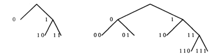
Fig. 2. Fibonacci trees, defined by $F(n) = \langle F(n-2), F(n-1) \rangle$ , for n = 4 and n = 5. Note that F(5) contains a copy of F(4) on its right side, and a copy of F(3) on its left side.
$$\begin{pmatrix} T_{0,0} & T_{0,10} & T_{0,11} \\ T_{10,0} & T_{10,10} & T_{10,11} \\ T_{11,0} & T_{11,10} & T_{111,11} \end{pmatrix} \begin{pmatrix} T_{00,00} & T_{00,01} & T_{00,10} & T_{00,110} & T_{00,111} \\ T_{01,00} & T_{01,01} & T_{01,10} & T_{01,110} & T_{01,111} \\ T_{10,00} & T_{10,01} & T_{10,10} & T_{10,110} & T_{10,111} \\ T_{111,00} & T_{111,01} & T_{111,110} & T_{111,110} & T_{111,111} \end{pmatrix} \tag{5} $$
It is also possible to consider multi-parameter tree families, each with a corresponding family of connection matrices.
Removing the restriction to complete, balanced binary trees has the effect of allowing termination of paths at different depths in the tree. Then the row and column labels of a connection matrix would have different lengths, so Eq. (4) could not be applied. This problem can be circumvented by formally extending the shorter string using multiple copies of a new symbol "2," until its length equals that of the larger string. Equation (4) is again applicable, although the decomposition matrix must be augmented by parameters $D_{p2}^{ab}$ and $D_{2a}^{ab}$ .
As a further refinement we may set $T_{\varepsilon\varepsilon}^{(a)} = 1$ , where $\varepsilon$ is the empty string, and we may add a final "2" to each string and set $D_{22}^{ab} = \delta_{ab} D^{\wedge (a)}$ , where $\delta_{ab}$ is the Kronecker delta. In this manner the basis values become part of the decomposition matrix. Thus the recursion parameters, the basis values, and the new parameters $D_{p2}^{ab}$ and $D_{2q}^{ab}$ can all be aggregated into one 4-index object $(D_{22}^{ab})$ .
Our basic equation (4), which now accommodates general lineage trees, can be rewritten with the recursion expanded as
$$T_{i_0i_1...i_n,\ j_0j_1...j_n}^{(a)} = \sum_{b_0} D_{i_0,j_0}^{a,b_0} \sum_{b_1} D_{i_1,j_1}^{b_0,b_1} ... \sum_{b_n} D_{i_n,j_n}^{b_{n-1},bn} \tag{6} $$
We observe that for i and j fixed, Eq. 6 is a sum (over $b_n$ ) of matrix products, and a given term in the sum over $\{b_o \ldots b_n\}$ is the (i, j) th element of a tensor product.
Equation (6) is fundamental in defining the meaning of the templates and lineage trees. Through the recursive division of templates into quadrants and of sets of neurons (contained in a lineage tree) into left and right subsets, the formalism embodies the principle of divide-and-conquer. The summation
makes it possible for several networks to be superimposed, a technique generally useful in network design.
The recursion equation approach to genetic neural networks has great expressive power. It allows networks to contain arbitrary interconnections, including cycles. It also encompasses replication, as demonstrated in the Appendix, suggesting applications to VLSI design where replication and hierarchy are fundamental.
2.2. Learning and Network Optimization
Current methods of learning with circuits or neural networks generally involve minimization of an objective function $E_{task}$ which characterizes the task to be learned. Standard techniques for accomplishing this include the Boltzman machine [5], back-propagation [19], and master/slave nets [11]. In applying these methods, one customarily uses the connection matrices T as independent variables. When recursion equations for genetic neural networks are used, however, it is the D-matrices which are the independent variables, and the objective function depends on them through the connection matrices: $E_{task}$ - $E_{task}$ (T(D)).
With this understanding, we can use simulated annealing or, if the connection matrix is of "feed-forward" type, back-propagation to search for the optimizing set of D-matrices.
For these optimization methods, T depends not only on D but also on the lineage tree. If a fixed family of lineage trees is chosen, depending, for example, on a single size parameter or "generation number" n, then $E_{task}$ - $E_{task}$ (T(D, n)). The goal is to minimize this quantity for some or all very large values of n, but only small values of n are available in practice due to the expense of optimizing the objective function for large connection matrices. But evaluating $E_{task}$ once is much cheaper than optimizing it and can therefore be done for much larger values of n, if there is reason to believe that T(D, n) might scale well.
For this reason we optimize the task performance on the first g generations of small networks. Thus we optimize
$$E_{task} = \sum_{n=1}^{g} E_{task} \left( T(D, n) \right) \tag{7}$$
so that a single D is forced to specify T at a variety of different sizes, and then we evaluate $E_{task}$ (T(D, n)) for $n \gg g$ . It is a remarkable fact that this $E_{task}$
$(T(D, n \gg g))$ can still be very low; in other words, that for optimization purposes Eq. (7) can approximate
$$E_{task} = \sum_{n=1}^{G \times g} E_{task} \left( T(D, n) \right) \tag{8} $$
This can only be done by finding and using scaling relationships, expressed in our case by the decomposition matrix D.
We wish to discourage learning by large scale memorization, i.e., by the formation of large look-up tables, because such procedures do not allow generalization. To control the amount of information which may be stored in D we add a parsimony constraint to $E_{task}$ . Several measures of parsimony are possible; the one which we have adopted in this paper is
$$E_{parsimony} = \sum_{abpa} V \left( D_{pq}^{ab} \right), \tag{9}$$
where V(D), the parsimony cost of each template entry, has three components: a cost $\lambda_1$ if D is nonzero, a cost $\lambda_2$ for each bit in a binary expansion of D, and a cost $\lambda_3|x|$ for an extra factor $2^x$ , where x is an integer, in the expression for D.
For efficiency of network evaluation, feed-forward networks may be encouraged by penalizing all but the feed-forward connections:
$$E_{feed-forward}(D,g) = \sum_{n=1}^{g} \sum_{\substack{ij \\ feedback}} |T_{ij}(D,n)|. \tag{10} $$
This term is of the same form as $E_{task}$ but is not nearly as task specific, depending only on the assignment of neurons to successive layers in the network. In our experiments, however, we simply truncated feedback connections to zero rather than penalizing them. Equation (10) could be modified to include all connections, thereby introducing a general sparseness constraint that favors less costly connectivity patterns in the final network.
The entire objective function employed in Section 3 is of the form
$$E(D) = E_{task}(D, g) + E_{parsimony} + \mu E_{feed-forward}(D, g), \quad (11)$$
which depends on g, $\lambda_1$ , $\lambda_2$ , $\lambda_3$ , and $\mu$ ,, and is to be minimized by simulated annealing.
2.3. Discussion
There are notable differences between the optimization method just described and others currently in use. The Boltzman machine learning rule, for example, is a local rule involving symmetric connections. Symmetric connections imply that there is an additional energy function, not present in our formulation, which depends on neuron activities rather than on synapse strengths and is minimized as the network runs. The back-propagation learning rule is a local rule originally restricted to feed-forward connections. Equation (6) can express asymmetric and non-feed-forward connections, and we will not impose an energy function which is minimized by neuron activities, so these restrictions on connectivity do not apply to genetic neural nets.
Genetic neural nets as described by Eq. (6), on the other hand, are not local. Non-local learning rules are required to express the structure which is present in the network.
Back-propagation has difficulty with generalization (see, e.g., Denker et al. [2]) and is very costly, if it does not actually fail, when scaled up to larger circuits [17]. We think that the basic reason for these scaling and generalization problems is the unstructured nature of the networks that can result from back-propagation. The use of a concise reparameterization of the space of connection matrices favors structured nets which scale.
Both back-propagation and the Boltzman machine involve gradient descent in the space of connection matrices for a neural network, but back-propagation may be the more practical algorithm, at least when it is restricted to feed-forward nets. (The case of non-feed-forward networks is dealt with by Lapedes and Farber [11] and by Pineda [16].) To compare our method to back-propagation, which allows one to compute $dT/dt \propto dE_{score}/dT$ efficiently for a feed-forward network, one need only obtain dT/dD analytically from Eq. (6) and follow gradients:
$$\frac{dD}{dt} \propto \frac{\partial E_{score}}{\partial D} = \sum \frac{\partial E_{score}}{\partial T} \frac{\partial T}{\partial D}.$$
Our experiments with this gradient descent method were much less successful than the experiments with simulated annealing reported in Section 3, owing perhaps to very local minima introduced by the parsimony constraint.
There is a body of recent work in theoretical computer science which supports the idea that parsimony is important to machine learning. We cite the work of Angluin [1], Haussler [4], and Rivest and Schapire [18]. We also mention the hand-designed structure in the networks of Scalettar and Zee [20] which leads to successful generalization. We expect parsimony and structure to be of increasing importance in studies of machine learning.
We use the genetic analogy in a fundamentally different way than does John Holland and colleagues in their work on "genetic algorithms" [6]. For Holland, genetics provides new ideas for searching, such as crossover, whereas we focus on parsimonious rules for constructing nets. We nevertheless expect that our approach would be enhanced by the use of crossover and his by more extensive use of parsimony.
3. EXPERIMENTS WITH THE CONTINUOUS CODE PROBLEM
We next describe the results of numerical simulations which were carried out to test the ideas presented in the previous section. We consider the following problem [14], illustrated in Fig. 3. Given a unary input $\chi$ , for example a 1-dimensional image with a single spot at position $\chi$ , the task is to compute a compressed code for $\chi$ in such a way that nearby $\chi$ 's have codes which are "nearby" in the sense that they differ by only a few bits. In other words, a small change in the input number corresponds to a small Hamming distance between the two output codes, a small Hamming distance between two code words corresponds to a small distance between the corresponding numbers (graceful degradation under codeword corruption-a kind of fault-tolerance), and in general the unsigned difference between two numbers is to be a monotonic function of the Hamming distance between the two codes.
This defines a "continuous code" problem which requires optimization of a feed-forward neural network with N input neurons equally spaced on the unit interval, $A = 2 \log N$ output neurons, and no interneurons, so that two unary inputs which are geometrically close to one another will produce two outputs which are close in the Hamming metric. The objective function for this task therefore relates geometric distance to Hamming distance,
$$E_{task}(o) = \frac{1}{N^2} \sum_{i,j=1}^{N} \left[ \left| \frac{i-j}{N} \right|^p - \frac{1}{A} \sum_{\alpha=1}^{A} \left( o_{\alpha i} - o_{\alpha j} \right)^2 \right]^2, \tag{12}$$
where oi-[ ] 0,1 is the value of the output neuron indexed by a when the input neurons are all clamped to zero except for the i th one, which is clamped to one. If only the i th input neuron is on, the column o*i describes the net's output and is thus the code word corresponding to input i. Likewise, each output neuron may be thought of as a "feature detector" in which case the row oa* is the feature to which it responds. Equation (12) is quartic in oai .
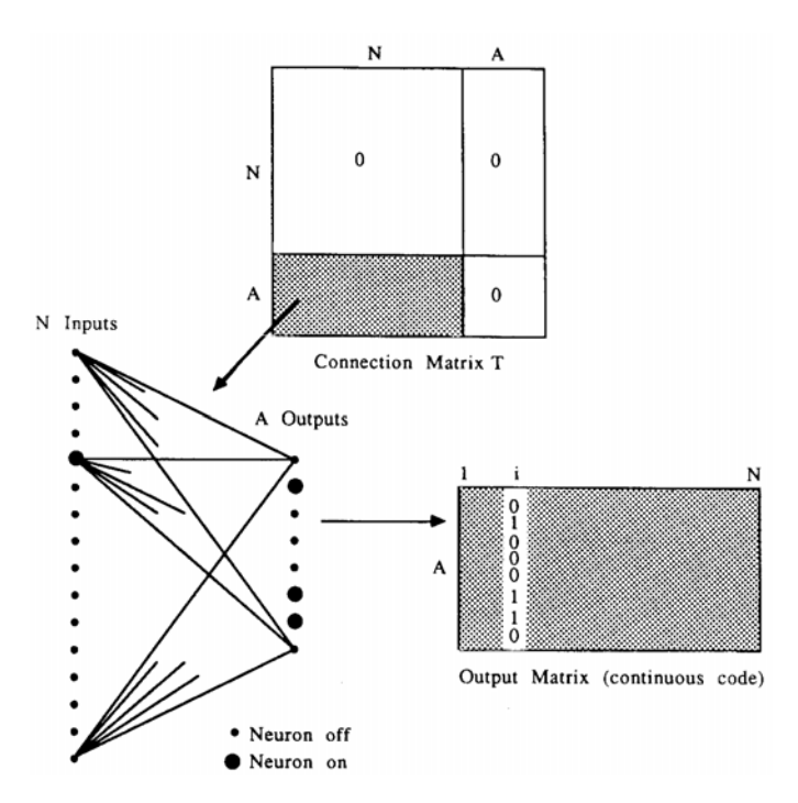
FIG. 3. The continuous coding task. A connection matrix of the form shown generates a feed-forward network. For each input i the network outputs are recorded in a column of the output matrix (or code matrix). The continuity of the output matrix is numerically evaluated by an objective function. Nearby values of i should generate nearby output codes if the objective function is to be minimized.
Because there are only N legal inputs to this network, the problem of generalization is not nearly as difficult as it could be for some other tasks. However, it is definitely nontrivial, since we will train the network for sizes N (and A = 2 log N) which are far smaller than those for which we will test the network. In fact the sizes of successive generations, indexed by an integer n, will be determined by N = 2n .
The energy function $E_{task}$ (o) in Eq. (12) becomes a function of T rather than o once we determine o(T). This involves running the network on each input i; that is, the input neurons are clamped to zero except for the i th one which is set to one. Then neuron values $s_i$ are repeatedly updated until they all stop changing. Various update rules can be employed; we use the update rule for discrete neurons
$$s_i(t+1) = \frac{1}{2} \left[ 1 + \operatorname{sgn}\left(\sum_j T_{ij} \, s_j(t)\right) \right]. \tag{13}$$
Whether the update is done synchronously (as in this equation) or asynchronously does not matter for a feed-forward net. In this way we obtain $E_{task}$ (T) which together with Eq. (6) defines $E_{task}$ (T(D, n)) which may be substituted into Eq. (7). Then the entire objective function E(D) is given by Eq. (11). We optimize E(D) by simulated annealing [10] using the Metropolis method [13] for updating each decomposition matrix element. The temperature schedule is determined by an initial temperature $t_{high}$ , a constant factor $f_{reduce}$ for reducing the temperature, a fixed number of accepted local moves required at each temperature, and an upper bound on the number of rejections allowed at a temperature which, if violated, terminates the run. Initially all decomposition matrix entries $D_{pq}^{ab}$ are zero.
Simulated annealing involves generating moves which alter the templates. A single move consists of changing one $D_{pq}^{ab}$ ; a sequence of moves repeatedly runs through all possible values of indices a, b, p, q. For the purpose of generating possible moves, each nonzero $D_{pq}^{ab}$ is represented in binary numbering as $D_{pq}^{ab} = m \times 2^x = \pm b_k b_{k-1} \dots b_o \times 2^x$ . The number of mantissa bits, k+1, varies and contributes to the parsimony cost, $V(D_{pq}^{ab}) = \lambda_1 + \lambda_2 k + \lambda_3 |x|$ , where $\lambda_1, \lambda_2, \lambda_3$ are input parameters.
Initially $D_{pq}^{ab}$ is zero so $V(D_{pq}^{ab})=0$ . The move from zero is to $\pm 1\times 2^{\circ}$ , $\pm 1\times 2^{-2}$ , or $\pm 1\times 2^{-4}$ , with all six choices equally likely. Subsequent moves serve to increase, decrease, or maintain the precision k, or set $D_{pq}^{ab}=0$ , all with equal probability. For example, if $D_{pq}^{ab}=101_2\times 2^{-3}$ , the precision is increased by moving to $1011_2\times 2^{-2}$ or $1001_2\times 2^{-4}$ , the precision is decreased by moving to $102\times 2^{-2}$ or $112\times 2^{-2}$ , and the precision is maintained by moving to $110_2\times 2^{-3}$ or $100_2\times 2^{-3}$ . Note some of these moves create trailing
zeroes in the mantissa; this is necessary to ensure there is a path to any number.
The lineage trees used are shown in Fig. 4; they contain N = 2n input neurons and A = 2 log N output neurons.
We record here the values of various parameters used in the optimization experiments. There were three families of decomposition matrices (index a and b ranged from 1 to 3 in ab Dpq ); this number was chosen to minimize computing costs and as a further hard parsimony constraint on the solutions. These three families were trained on generations 2 through 5 and tested on generations 6 through 8; . the temperature started at thigh = 0.05 and dropped by factors of , freduce = 0.8 each time 500 update changes were
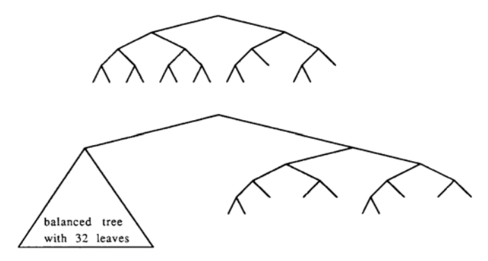
FIG. 4. The lineage trees used in the experiments consist of two subtrees: a balanced binary tree of size N for the input neurons and an almost balanced binary tree of size A for the output neurons. An almost balanced tree of size M consists of almost balanced subtrees of size [M/2] and [M/2]. Trees for A = 6 and A = 10 are shown.
accepted, stopping only when 20,000 rejections were required to get these 500 acceptances; the parsimony weights were 1 = 0.00032, 2 = 0.000005, and 3 = 0.000005.
At any value of p we can compare the genetic neural network method's performance to simulated annealing considered as an optimization method operating directly on the space of all one-layer feed-forward connection matrices. The simplest experiment involves comparing GNN and simulated annealing for the sequence of slightly different tasks parameterized by p (Eq. (12)) by computing the ratio of scores
$$\frac{E_{genetic}(p,n)}{\langle E_{control}(p,n)\rangle},$$
where the control score is averaged over three independent runs. Twelve runs for each of several values of the task parameter p are shown in Fig. 5. During the GNN simulated annealing procedure, genetic descriptions are sometimes found which scale better than any later configuration, but are thrown away. This phenomenon may be called "overlearning" and we do not entirely understand it, though it is similar to many dynamical systems in which a trajectory will linger near one attractor before settling into another. To take advantage of this phenomenon, we test the genetic description on size n = 6 (one size larger than the training set) after each 500 update acceptances. We continually keep the genetic description with the lowest score so far on size n = 6. This stored decomposition matrix is the output of the GNN optimization procedure; the decomposition matrix chosen is often the last one reached in the course of annealing. Since the
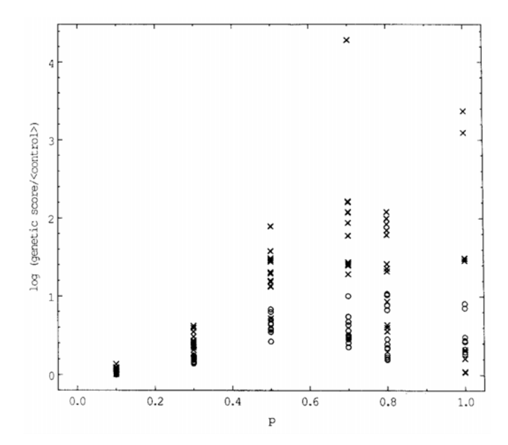
Fig. 5. The ratio of scores of genetically optimized nets and of control experiments involving simulated annealing of unstructured nets, as a function of a parameter p appearing in the continuous coding task. Control experiments are averaged over three runs. For each p, twelve GNN runs are shown. Crosses show results for n = 5, the largest training size for the genetic optimization (but very infrequent evaluations are also made at size n = 6 to prevent overlearning, as described in the text). Open circles show results for n = 8, where the network is obtained by pure extrapolation without any further training.
evaluation on size n = 6 is performed very infrequently compared to the training evaluation on sizes n = 2 through 5, it adds almost no computational expense.
The average of control experiment scores is empirically well behaved: the associated standard deviation is only a few percent of the mean. As shown in Fig. 5, however, the genetic scores vary by a factor of as much as 30 between good runs and bad runs, both of which happen frequently. To filter out the worst runs we consider a set of four successive runs and choose the output of the genetic learning procedure to be the best decomposition matrix in the set, as judged by its performance at n = 6. It is this filtered genetic description which we examine for scaling; its relative score, averaged over three sets of runs, is
$$R(p,n) = \frac{\left\langle \min_{4 \text{ runs}} E_{\text{genetic}}(p,n) \right\rangle_{3 \text{ sets of runs}}}{\left\langle E_{\text{control}}(p,n) \right\rangle_{3 \text{ runs}}},$$
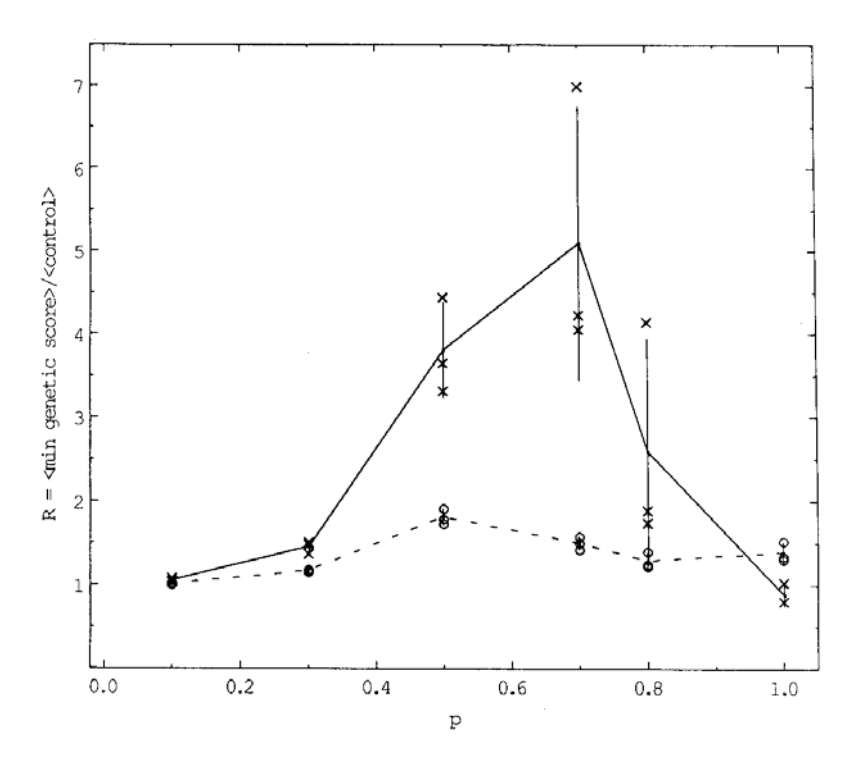
FIG. 6. The ratio of filtered scores for genetic neural nets and of the control experiments as described in Fig. 5. All GNN experimental results are averaged over three sets of four runs; within each set of four runs the best result for n = 6 is selected. This procedure reliably filters
out the poor runs present in Fig. 5. Dotted lines show results for n = 5, the largest training size for the genetic optimization. Solid lines show results for n = 8, demonstrating scaling without further training or filtering.
This quantity is shown by the dotted line in Fig. 6 for generation n = 5, the last generation for which the decomposition matrices were trained, and for which N = 32 and A = 10. The associated variance, and the relative scores for each run,
$$\frac{\min_{4 \text{ runs}} E_{\text{genetic}}(p, n)}{\left\langle E_{\text{control}}(p, n) \right\rangle_{3 \text{ runs}}},$$
are also shown as a function of p in this figure. Next, the recursion relation (6) is used to extrapolate far beyond the training set to generation n = 8, where the network size parameters are N = 256 and A = 16. The resulting large network has had no training at all on any inputs of size N = 256, and yet performs well as indicated by the solid line in Fig. 6, with associated data points and variances. We note that the comparison with the control experiments is best near p = 0 and p = 1, and is not as good near p = 0.5.
This may indicate that the solution is intrinsically more complicated near p = 0.5. We also report that, as the size n is increased past 5, the p = 0.5 control scores decline slowly and the absolute GNN scores rise very slowly. Thus there is nontrivial scaling behavior even for p = 0.5.
One may also study generalization along the scale axis in more detail as in Table I, where (min4 runs Egenetic (p, n)) and (Econtrol (p, n)) (each averaged over three trials, as before) are displayed as a function of n, for p = 0.1. At p = 0.1 and n 5 the control scores are relatively flat, so we report genetic scores for sizes considerably beyond the sizes for which we can afford to do the control experiments. The relatively flat GNN scores extend well past the training set size; this demonstrates successful scaling. In addition, it is possible to come considerably closer to the control scores by using a slower GNN annealing schedule than that used in Table I and Figs. 5 and 6.
On a Multiflow Trace 7/200, the computing time for a single run of the control experiment for n = 8 was 4.4 CPU-h, whereas the GNN method required an initial investment of 18.6 h (including four runs for the filtering step) to get the recursion relation for sizes n = 2 through 5, and an extra half second to extrapolate the recursion relation to obtain a connection matrix for n = 8. The initial GNN investment time may not yet be minimal, because the continuous coding score energy is completely recomputed at each move in the GNN procedure, but incrementally recomputed for each move in the control experiment. It is possible that incremental GNN evaluation would be faster. Nevertheless, for larger sizes the GNN method becomes much faster than the control method because only the relatively small extrapolation time changes; it is not necessary to recompute the recursion relation.
Table I shows further comparative timing data which demonstrate a great advantage for the GNN method: not only do the asymptotically GNN timings increase linearly in $N = 2^n$ , compared to the control timings which are increasing quadratically, but there is an additional constant factor of about $10^2$ which favors the GNN timings. The control experiment timings are minimal, since they assume that the required number of acceptances and the allowed number of rejections in the control experiment's annealing procedure scale linearly with N, which is an optimistic assumption. Also, unlike the control timings, the GNN timings are much smaller than the quadratically increasing time required to perform a single evaluation of the energy function; thus only the time to compute the network, and not the time to exhaustively test it, is reported. All reported timings are averages over three runs. We conclude that the GNN learning method is asymptotically much faster than the control method.
We present an example of a decomposition matrix and its n = 3 and n = 6 output matrices $o_{ai}$ which were found by our optimization procedure.
The example is for the case p = 0.1 and has scores of 0.0971 for n = 3 and 0.1423 for n = 6, which are good. For clarity of display, blanks indicate matrix entries with value 0. For n = 3, o is
| 1 | 1 | 1 | 1 | ) | |||
|---|---|---|---|---|---|---|---|
| 1 | 1 | 1 | 1 | ||||
| 1 | 1 | 1 | 1 | ||||
| 1 | 1 | 1 | 1 | ||||
| 1 | 1 | 1 | 1 | ||||
| 1 | 1 | 1 | 1 |
and for n = 6 it is
| (11111111 | L | 11111111 | 111111111 | 1111111 | ) |
|---|---|---|---|---|---|
| 1111 | 11111111 | 1111 1111 | 1111 | 1111 | 1111 |
| 11111111 | 11111111 | 1 | 111111111 | 111111 | |
| 11111111 | 11111111111111 | 111 1 | 1111111 | ||
| 1111 | 1111 1111 | 1111 | 1111 1111 | 1111 | 1111 |
| 1111 | 111111111111 | 111111111 | 111111 | ||
| 11111111111111 | 11 | 111111111 | 1111111 | ||
| 1111 | 1111 - 11 | 11 11111111 | 1111 | 1111 | 1111 |
| 111111 | 1111111111 | 1 | 111111111 | 111111 | |
| 11111111 | 111111 | 11 1111 | 1111 1 | 1111111 | |
| 1111 | 1 1111 11 | 11 1111 | 1111 1111 | 1111 | 1111 |
| (1111 | 11 1 11 1 1 1 | 1 11 1 11 1 | 11 11 1 1 | 11 1 11 | 1 11 |
In agreement with results of our earlier investigations [14] at small p, all of the features (the rows of these o matrices) are Walsh functions. (To make this identification we must replace zero entries with -1, or use output neurons with values $\pm$ 1 instead of 0 and 1.) The Walsh functions are a standard orthogonal set of basis functions [3] used in the Walsh transform, analogous to trigonometric basis functions for the Fourier transform. Algorithms for computing the Walsh functions are given in [3] and below.
Extending the $\tau_a(n)$ notation of Eq. (2) to include the 3 X 3 matrices $D_{**}^{ab}$ , where the * subscripts take values "0," "1," or "2" as described in
$\label{eq:TABLE I} TABLE\ I$ Scaling and Timing, p=0.1
| Size n | Score | CPU time (s) | ||
|---|---|---|---|---|
| $N = 2^n, A = 2 n$ | GNN | Anneal T | GNN | Anneal T |
| 2-5 a | $0.1381 \pm 0.0012$ | $0.1364 \pm 0.0001$ | 16766 b | $214 \pm 25$ |
| 6 | $0.1431 \pm 0.0023$ | $0.1394 \pm 0.0001$ | $0.1 \pm 0.05$ | $793 \pm 48$ |
| 7 | $0.1466 \pm 0.0040$ | $0.1400 \pm 0.0001$ | $0.2 \pm 0.05$ | $3548 \pm 136$ |
| 8 | $0.1479 \pm 0.0034$ | $0.1400 \pm 0.0001$ | $0.5 \pm 0.05$ | $15902 \pm 123$ |
| 9 | $0.1477 \pm 0.0031$ | c | $1.2 \pm 0.05$ | $64000^d$ |
| 10 | $0.1474 \pm 0.0033$ | С | $2.7 \pm 0.05$ | С |
| 11 | $0.1466 \pm 0.0030$ | С | $6.0 \pm 0.17$ | С |
| 12 | $0.1462 \pm 0.0026$ | С | $12.9 \pm 0.10$ | С |
| 13 | $0.1460 \pm 0.0023$ | c | $28.2 \pm 0.05$ | c |
<sup>aScores are for size 5.
Section 2.1, we may express the learned recursion relations as
<sup>bMultiply by four to account for filtering. Includes training on sizes 2-5.
<sup>cNot computed due to expense.
<sup>dEstimated.
$$\tau_{0}(n+1) = \begin{pmatrix} 0 & 0 & 0 \\ \tau_{1}(n) - \tau_{2}(n) & 0 & 0 \\ \hline 0 & 0 & 0 \end{pmatrix}$$
$$\tau_{1}(n+1) = \begin{pmatrix} -\tau_{1}(n) & \frac{1}{2}\tau_{1}(n) & 0 \\ \underline{\tau_{1}(n)} & \tau_{1}(n) & 0 \\ -\tau_{1}(n) & -2\tau_{1}(n) & \frac{1}{2}\tau_{1}(n) \end{pmatrix}$$
$$\tau_{2}(n+1) = \begin{pmatrix} 0 & 0 & 0 \\ \frac{5}{2}\tau_{2}(n) & -3\tau_{2}(n) & \tau_{2}(n) \\ 0 & -4\tau_{2}(n) & 2\tau_{2}(n) \end{pmatrix} \tag{14} $$
for all $n \ge -1$ . Also $\tau_a(-1) = 1$ , for all a.
Here the $3 \times 3$ matrices are to be converted to $2 \times 2$ matrices in accordance with the shape of the lineage tree as well as its maximum depth, n, in the manner determined by Eq. (6). The horizontal and vertical bars in Eq. (14) separate the $2 \times 2$ matrices from the terminating values $D_{p2}^{ab}$ , $D_{2q}^{ab}$ and $D_{22}^{aa}$ .
Note the great simplicity of these recursion relations. They may be understood fairly easily: the $\tau_o$ family of matrices, which serves as the final network connection matrix, is specialized to eliminate all but the feed-forward connections from input neurons to output neurons and thereby gain parsimony. The Walsh functions are implicit in the expression for $\tau_1$ (n+1), for they are generated by the tensor product
$$T_{i_1...i_n, j_1...j_n} = M_{i_1, j_1} M_{i_2, j_2} ... M_{i_n, j_n}$$
where
$$M = \begin{pmatrix} -1 & 1 \\ 1 & 1 \end{pmatrix}, \quad M \otimes M = \begin{pmatrix} 1 & -1 & -1 & 1 \\ -1 & -1 & 1 & 1 \\ -1 & 1 & -1 & 1 \\ 1 & 1 & 1 & 1 \end{pmatrix}, \dots$$
which is, in our notation,
$$\tau_{1}(n+1) = \begin{pmatrix} -\tau_{1}(n) & \tau_{1}(n) & 0 \\ \tau_{1}(n) & \tau_{1}(n) & 0 \\ \hline 0 & 0 & \tau_{1}(n) \end{pmatrix}$$
for $N = A = 2^n$ . The remaining entries of $\tau_1$ and $\tau_2$ may be regarded as adjustments for the fact that A is neither large nor a power of 2 in the continuous coding problem.
A second example illustrates the dominant GNN behavior for $p \ge 0.8$ . This set of solutions generates output matrices which appear to be nearly optimal for p = 1, and are not optimal for $p \le 0.9$ but score well enough and are very simple. We exhibit one particularly parsimonious set of recursion relations which was learned for p = 1. The n = 3 output matrix o is
$$\begin{pmatrix} 1 & & & & & \\ 1 & 1 & 1 & & & & \\ 1 & 1 &$$
and larger sizes also result in triangular matrices, scaled up. The triangular o matrices show that the network computes a kind of unary code in which the position of the single input neuron which is turned on is linearly mapped into the position of the boundary between blocks of on and off output neurons. The recursion relations themselves are
$$\tau_0(n+1) = \begin{pmatrix} 0 & 0 & 0 \\ \tau_1(n) & 0 & 0 \\ \hline 0 & 0 & 0 \end{pmatrix}$$
$$\tau_{1}(n+1) = \begin{pmatrix} \tau_{1}(n) & \tau_{2}(n) & 0 \\ 0 & 8\tau_{1}(n) & 0 \\ \hline 0 & \tau_{2}(n) & 0 \end{pmatrix}$$
$$\tau_{2}(n+1) = \begin{pmatrix} \tau_{2}(n) & \frac{1}{2}\tau_{2}(n) & 0 \\ \hline \tau_{2}(n) & \tau_{2}(n) & 0 \\ \hline \tau_{2}(n) & \tau_{2}(n) & -6\tau_{2}(n) \end{pmatrix} \tag{15} $$
for all $n \ge -1$ . Also $\tau_a(-1) = 1$ , for all a.
Once again the $\tau_0$ family is specialized to eliminate all but feed-forward connections. Now $\tau_2$ is specialized to create rectangular blocks of negative matrix entries, and $\tau_1$ is specialized to make triangular submatrices. (The thresholding operation for the output neurons sent zero or positive input sums to + 1 output values and negative input sums to zero output values; the learned solutions rely on this treatment of the special zero-input-sum case.) The coefficients 8, 1/2, and 6 could be set to unity without affecting performance.
4. EXTENSIONS OF THE GNN THEORY
The purpose of this section is to outline several fundamental extensions of the GNN theory presented in Section 2. The experimental investigation of these ideas is left to future research.
4.1. Structured Trees
The families of lineage trees defining the address of a neuron have had a regular structure, but their structures have been imposed as part of the task. Can these structures be learned, and what would be gained by doing so? The principal advantage would be that the optimization procedure would have greater freedom to choose its own mapping of the problem onto circuit elements, i.e., to develop its own representation of the problem.
The objective functions of Section 2.2 depend on the decomposition matrices and on the lineage trees. What we shall do here is provide a recursive description of families of lineage trees in terms of new parameters analogous to those occurring in the decomposition matrices.
The nodes in an infinite binary tree can be indexed, or addressed, by strings $i_1 \dots i_n$ , of 0's and 1's. $\tau_o$ each node in the tree we assign a variable $L_{i_1 \dots i_n}$ which is 1 if that node occurs in the present lineage tree, and zero otherwise. $L_{i_1 \dots i_n}$ will be determined by a set of real weights $W_{i_1 \dots i_n}$ . If $W_{i_1}$ is among the N largest weights in the tree, then $L_{i_1 \dots i_n} = 1$ and the i th node is in the tree. Otherwise it is zero and the node is not in the tree. This procedure can be expressed as the minimization of
$$E_{tree}(L) = \left(\sum_{n=1}^{\infty} \sum_{i_1 \dots i_n} L_{i_1 \dots j_n} - N\right)^2 - \sum_{n=0}^{\infty} \sum_{i_1 \dots i_n} L_{i_1 \dots i_n} - W_{i_1 \dots i_n}. \tag{16} $$
In analogy with Eq. (4) for the decomposition matrices, we can now write a recursion relation for the weights,
$$W_{i_1...i_n}^a = \sum_{b=1}^B \omega_{i_1}^{ab} W_{i_2...i_n}^b \quad (n \ge 1). \tag{17} $$
The set of weights which specify the desired lineage tree can be taken to be $W^1_{i_1...i_n}$ . As in the case of the number of connection strength templates, if B is small then the lineage tree is structured.
We give an example. Consider the class of almost balanced lineage trees used in our experiments and described in Fig. 4. Figure 7 gives an assignment of weights $W_{i_1 \ldots i_n}$ to the infinite binary tree which gives this class of lineage trees. The figure also shows a set of weights $W_{i_1 \ldots i_n}$ which are needed in the recursion relation for $W_{i_1 \ldots i_n}$ . To produce these weights,

FIG. 7. A portion of the infinite structured lineage tree determined by weights generated in Eqs. (17) and (18).
one uses Eq. (17) with the hand-designed coefficients
$$\omega_0^{11} = \frac{1}{2}, \quad \omega_1^{11} = \frac{1}{2}, \quad \omega_0^{12} = \frac{1}{2}, \quad W_{\varepsilon}^{1} = 1$$
$$\omega_0^{23} = 1, \quad \omega_1^{23} = 1, \quad W_{\varepsilon}^{2} = 0$$
$$\omega_0^{33} = \frac{1}{4}, \quad \omega_1^{33} = \frac{1}{4}, \quad W_{\varepsilon}^{3} = \frac{1}{4}. \tag{18} $$
A11 other $\omega_p^{ab}$ are zero.
4.2. Function Similarity Matrix
Consider a collection of templates. The operation of substituting one template for another in a decomposition matrix would, with high probability, be counterproductive (result in a lower score). However, if two templates b and c are known on the basis of past experience to perform a similar function, then the substitution of c for b should improve the score with probability approaching one half. How can we discover and use such similarities?
If a decomposition matrix element $D_{2q}^{ab}$ is nonzero, the collection of indices a, p, q, specifies a place where b can occur. We call the triple a, p, q a context of b. If c can be substituted for b in one context, we propose that c is similar to b and can also be substituted in another context.
We introduce slowly changing variables $S_{bc}$ C=- [0,1] which measure the degree of similarity between b and c. The matrix S is called the function similarity matrix. The effect of $S_{bc}$ , on the optimization procedure will be expressed by a new contribution to the objective function. We pick this to be of the form:
$$E_{FSM}(D,S) = -v \sum_{\substack{bc \\ \text{substitutions}}} \sum_{\substack{pqa \\ \text{contexts}}} D_{pq}^{ab} D_{pq}^{ac} S_{bc}. \tag{19} $$
This has the following effects: $S_{bc}$ , increases when templates b and c are in competition for the same position, and template c will be introduced into competition with template b when $S_{bc} > 0$ . The efficacy of this new term may be measured by varying its Lagrange multiplier and observing the effect on performance.
Our experiments so far have not involved sufficiently many templates to justify the use of the function similarity matrix. It may be thought of as a means of organizing a large library of templates for use in learning.
4.3. GNN Summary
As augmented by structured trees and the function similarity matrix, we may summarize the full GNN approach to learning as follows:
(1)
$$T_{i,j}^{(a)} = \sum_{b} D_{i_1 j_1}^{ab} T_{i',j'}^{(b)}$$
, $(i = i_1 ... i_n; i' = i_2 ... i_n)$
(2) $W_i^a = * \sum_{b} \omega_{i_1}^{ab} W_{i'}^b$ ;
choose the largest $N$ weights $W_i^1$ to get a lineage tree
(3) $E(D) = \sum_{generations n} E_{task} (T(D, n)) + \sum_{abpq} V(D_{pq}^{ab})$
$-* v \sum_{bc} \sum_{paa} D_{pq}^{ab} D_{pq}^{ac} S_{bc}$ .
The unstarred expressions have been tested by numerical experiments whose results are reported in this paper. The findings on the test problem considered may be summarized as follows: (a) genetic neural nets permit generalization by scaling, in that nets trained on small problems continue to score well on much larger versions of the same problem, and (b) the computation with structured nets is more efficient than direct optimization of connection matrices to a degree that increases with problem size. Equation (20) is our present formulation of genetic neural networks, and it is subject to change in response to new experiments.
APPENDIX: RECURSIVE DESCRIPTIONS OF GRIDS OF DIMENSION 2 AND 3
In the following recursion equation, $\tau_l(n)$ specifies the connection matrix for a 2-dimensional toroidal grid whose neurons are numbered in the hierarchical zig-zag order shown in Fig. 8(a). The dimensions of the grid are $2^{2[n/2]} \times 2^{2[n/2]}$ .
The relationship between the templates is shown as a graph in Fig. 8(b). a and b are independently controllable weights on the final grid connections in the x and y directions, respectively, allowing one to describe
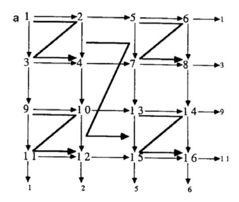
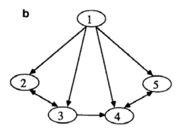
FIG. 8. (a) 2 D toroidal grid: Connection pattern and ordering of sites. Note periodic boundary conditions for $4 \times 4$ grid. (b) 2 D grid: Graph of dependencies between templates.
anisotropic, homogeneous grids. The recursion equation is
$$\tau_{1}(n+1) = \begin{pmatrix} \tau_{2}(n) + \tau_{3}(n) + \tau_{5}(n), \tau_{4}(n) \\ \tau_{4}(n), \tau_{2}(n) + \tau_{3}(n) + \tau_{5}(n) \end{pmatrix} \qquad \tau_{1}(0) = 0, \tau_{2}(n+1) = \begin{pmatrix} \tau_{3}(n) & 0 \\ 0 & \tau_{3}(n) \end{pmatrix}, \qquad \tau_{2}(0) = 0, \tau_{3}(n+1) = \begin{pmatrix} \tau_{2}(n) & \tau_{4}(n) \\ 0 & \tau_{2}(n) \end{pmatrix}, \qquad \tau_{3}(0) = 0, \tag{21}$$
$$\tau_{4}(n+1) = \begin{pmatrix} \tau_{5}(n) & 0 \\ 0 & \tau_{5}(n) \end{pmatrix}, \qquad \tau_{4}(0) = a, \tau_{5}(n+1) = \begin{pmatrix} 0 & 0 \\ \tau_{4}(n) & 0 \end{pmatrix}, \qquad \tau_{5}(0) = b,$$
for all $n \ge 0$ .
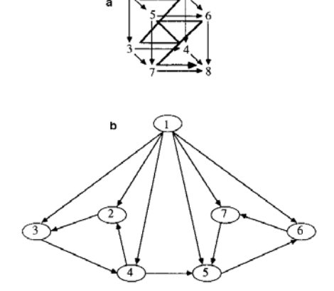
Fig. 9. (a) 3D grid: Local ordering of sites. (b) 3D grid: Template dependency graph.
A similar set of templates specifies three-dimensional toroidal grids as in Fig. 9. In this case the recursion equations are
$$\tau_{1}(n+1) = \begin{pmatrix} \tau_{2}(n) + \tau_{3}(n) + \tau_{4}(n) + \tau_{6}(n) + \tau_{7}(n), \tau_{5}(n) \\ \tau_{5}(n), \tau_{2}(n) + \tau_{3}(n) + \tau_{4}(n) + \tau_{6}(n) + \tau_{7}(n) \end{pmatrix} \tau_{1}(0) = 0,$$
$$\tau_{2}(n+1) = \begin{pmatrix} \tau_{3}(n) & 0 \\ 0 & \tau_{3}(n) \end{pmatrix}, \qquad \tau_{2}(0) = 0,$$
$$\tau_{3}(n+1) = \begin{pmatrix} \tau_{4}(n) & 0 \\ 0 & \tau_{4}(n) \end{pmatrix}, \qquad \tau_{3}(0) = 0,$$
$$\tau_{4}(n+1) = \begin{pmatrix} \tau_{2}(n) & \tau_{5}(n) \\ 0 & \tau_{2}(n) \end{pmatrix}, \qquad \tau_{4}(0) = 0, \tag{22} $$
$$\tau_{5}(n+1) = \begin{pmatrix} \tau_{6}(n) & 0 \\ 0 & \tau_{6}(n) \end{pmatrix}, \qquad \tau_{5}(0) = a, \tau_{6}(n+1) = \begin{pmatrix} \tau_{7}(n) & 0 \\ 0 & \tau_{7}(n) \end{pmatrix}, \qquad \tau_{6}(0) = b, \tau_{7}(n+1) = \begin{pmatrix} 0 & 0 \\ \tau_{5}(n) & 0 \end{pmatrix}, \qquad \tau_{7}(0) = c,$$
for all $n \ge 0$ .
REFERENCES
- D. ANGLUIN, "Queries and Concept Learning," Machine Learning, Vol. 2, pp. 319-342 (1988).
- J. DENKER, D. SCHWARTZ, B. WITTNER, S. SOLLA, R. HOWARD, AND L. JACKEL, Automatic learning, rule extraction, and generalization, Complex Systems 1, (1987), 922.
- R. C. GONZALES AND P. WINTZ, "Digital Image Processing," pp. 111-121, 2nd Ed., Addison-Wesley, Reading, MA, 1987.
- D. HAUSSLER, "Quantifying Inductive Bias in Concept Learning," Artifical Intelligence 36, (1988) 221.
- G. E. HINTON AND T. J. SEJNOWSKI, "Learning and Relearning in Boltzman Machines," in "Parallel Distributed Processing" D. Rumelhart and J. McClelland, (Eds.) Vol. 1, Chap. 7, MIT Press, Cambridge, MA, 1986.
- J. H. HOLLAND, "Escaping Brittleness": The Possibilities of General-Purpose Algorithms Applied to Parallel Rule-Based Systems, "Machine Learning II" (R. Michalski, J. Carbonell, and T. Mitchell Eds.) Chap. 20, Morgan Kaufmann, Los Altos, CA, 1986.
- J. J. HOPFIELD, Neural networks and physical systems with emergent collective computational abilities, Proc. Nat. Acad. Sci. U.S.A. 79, April (1982) 2558.
- J. J. HOPFIELD AND D. W. TANK, "Neural" computation of decisions in optimization problems, Biol. Cybernet. 52 (1985) 152.
- E. R. KANDEL and J. H. SCHWARTZ (Eds.) "Principles of Neural Science," p. 87, 2nd Ed., Elsevier, New York, 1985.
- S. KIRKPATRICK, C. D. GELATT, JR., AND M. P. VECCHI, Optimization by simulated annealing, Science 220, May (1983), 4598.
-
- A. LAPEDES AND R. FARBER, Programming a massively parallel, computation universal system: Static behavior, in "Neural Networks for Computing, Proceedings. Snowbird, Utah" (J. Denker, Ed.), Amer. Inst. Phys., New York, 1986, pp. 283-298.
-
- B. LEWIN, Units of transcription and translation: Sequence components of heterogeneous nuclear RNA and messenger RNA, Cell 4 (1975), Tables 6 and 7.
- N. METROPOLIS, A. ROSENBLUTH, M. ROSENBLUTH, A. TELLER, AND E. TELLER, Equation of state calculations by fast computing machines, J. Chem. Phys. 21(1953), pp. 1087-1092.
- E. MJOLSNESS AND D. H. SHARP, A preliminary analysis of recursively generated networks, in "Neural Networks for Computing, Proceedings, Snowbird, Utah" (J. Denker, Ed.), Amer. Inst. Phys., New York, 1986.
- E. MJOLSNESS, D. H. SHARP, AND B. K. ALPERT, Recursively generated neural networks, in "Proceedings, IEEE First Annual International Conference on Neural Networks," IEEE, New York, 1987.
- F. J. PINEDA, Generalization of backpropagation to recurrent and high-order networks, in "Neural Information Processing Systems" (D. Z. Anderson, Ed.), Amer. Inst. Phys. NY, (1988) pp 602-611.
- D. C. PLAUT, S. J. NOWLAN, AND G. E. HINTON, "Experiments on Learning by Back Propagation," Technical Report CMU-CS-86-126, Carnegie-Mellon University, 1986.
- R. L. RIVEST AND R. E. SHAPIRE, Diversity-based inference of finite automata, in "28th Annual Symposium" on Foundations of Computer Science, 1987."
- D. E. RUMELHART, G. E. HINTON, and R. J. WILLIAMS, "Learning Internal Representations by Error Propagation," in "Parallel Distributed Processing" (D. Rumelhart and J. McClelland, Eds.) Vol. 1, Chap. 8, MIT Press, Cambridge, MA, 1986.
-
- R. SCALETTAR AND A. ZEE, "Perception of Left and Right by a Feed Forward Net," Technical Report NSF-ITP-87-49, Institute for Theoretical Physics, Santa Barbara, 1987.