title: Natural Evolution Strategies url: http://arxiv.org/abs/1106.4487v1

Natural Evolution Strategies

Daan Wierstra daan.wierstra@epfl.ch

Laboratory of Computational Neuroscience, Brain Mind Institute Ecole Polytechnique F´ed´erale de Lausanne (EPFL) ´ Lausanne, Switzerland

Tom Schaul tom@idsia.ch Tobias Glasmachers tobias@idsia.ch Yi Sun yi@idsia.ch J¨urgen Schmidhuber juergen@idsia.ch

Istituto Dalle Molle di Studi sull'Intelligenza Artificiale (IDSIA) University of Lugano (USI)/SUPSI Galleria 2, 6928, Lugano, Switzerland

Editor: unknown

Abstract

This paper presents Natural Evolution Strategies (NES), a recent family of algorithms that constitute a more principled approach to black-box optimization than established evolutionary algorithms. NES maintains a parameterized distribution on the set of solution candidates, and the natural gradient is used to update the distribution's parameters in the direction of higher expected fitness. We introduce a collection of techniques that address issues of convergence, robustness, sample complexity, computational complexity and sensitivity to hyperparameters. This paper explores a number of implementations of the NES family, ranging from general-purpose multi-variate normal distributions to heavytailed and separable distributions tailored towards global optimization and search in high dimensional spaces, respectively. Experimental results show best published performance on various standard benchmarks, as well as competitive performance on others.

Keywords: Natural Gradient, Stochastic Search, Evolution Strategies, Black-box Optimization, Sampling

1. Introduction

Many real world optimization problems are too difficult or complex to model directly. Therefore, they might best be solved in a 'black-box' manner, requiring no additional information on the objective function (i.e., the 'fitness' or 'cost') to be optimized besides fitness evaluations at certain points in parameter space. Problems that fall within this category are numerous, ranging from applications in health and science (Winter et al., 2005; Shir and B¨ack, 2007; Jebalia et al., 2007) to aeronautic design (Hasenj¨ager et al., 2005; Klockgether and Schwefel, 1970) and control (Hansen et al., 2009).

Numerous algorithms in this vein have been developed and applied in the past fifty years (see section 2 for an overview), in many cases providing good and even near-optimal solutions to hard tasks, which otherwise would have required domain experts to hand-craft solutions at substantial cost and often with worse results. The near-infeasibility of finding globally optimal solutions requires a fair amount of heuristics in black-box optimization algorithms, leading to a proliferation of sometimes highly performant yet unprincipled methods.

In this paper, we introduce Natural Evolution Strategies (NES), a novel black-box optimization framework which is derived from first principles and simultaneously provides state-of-the-art performance. The core idea is to maintain and iteratively update a search distribution from which search points are drawn and their fitness evaluated. The search distribution is then updated in the direction of higher expected fitness, using ascent along the natural gradient.

1.1 Continuous Black-Box Optimization

The problem of black-box optimization has spawned a wide variety of approaches. A first class of methods was inspired by classic optimization methods, including simplex methods such as Nelder-Mead (Nelder and Mead, 1965), as well as members of the quasi-Newton family of algorithms. Simulated annealing (Kirkpatrick et al., 1983), a popular method introduced in 1983, was inspired by thermodynamics, and is in fact an adaptation of the Metropolis-Hastings algorithm. More heuristic methods, such as those inspired by evolution, have been developed from the early 1950s on. These include the broad class of genetic algorithms (Holland, 1992; Goldberg, 1989), differential evolution (Storn and Price, 1997), estimation of distribution algorithms (Larra˜naga, 2002), particle swarm optimization (Kennedy and Eberhart, 2001), and the cross-entropy method (Rubinstein and Kroese, 2004).

Evolution strategies (ES), introduced by Ingo Rechenberg and Hans-Paul Schwefel in the 1960s and 1970s (Rechenberg and Eigen, 1973; Schwefel, 1977), were designed to cope with high-dimensional continuous-valued domains and have remained an active field of research for more than four decades (Beyer and Schwefel, 2002). ESs involve evaluating the fitness of real-valued genotypes in batch ('generation'), after which the best genotypes are kept, while the others are discarded. Survivors then procreate (by slightly mutating all of their genes) in order to produce the next batch of offspring. This process, after several generations, was shown to lead to reasonable to excellent results for many difficult optimization problems. The algorithm framework has been developed extensively over the years to include self-adaptation of the search parameters, and the representation of correlated mutations by the use of a full covariance matrix. This allowed the framework to capture interrelated dependencies by exploiting the covariances while 'mutating' individuals for the next generation. The culminating algorithm, covariance matrix adaptation evolution strategy (CMA-ES; Hansen and Ostermeier, 2001), has proven successful in numerous studies (e.g., Friedrichs and Igel, 2005; Muller et al., 2002; Shepherd et al., 2006).

While evolution strategies prove to be an effective framework for black-box optimization, their ad hoc procedures remain heuristic in nature. Thoroughly analyzing the actual dynamics of the procedure turns out to be difficult, the considerable efforts of various researchers notwithstanding (Beyer, 2001; Jebalia et al., 2010; Auger, 2005). In other words, ESs (including CMA-ES), while powerful, still lack a clear derivation from first principles.

1.2 The NES Family

Natural Evolution Strategies (NES) are well-grounded, evolution-strategy inspired blackbox optimization algorithms, which instead of maintaining a population of search points, iteratively update a search distribution. Like CMA-ES, they can be cast into the framework of evolution strategies.

The general procedure is as follows: the parameterized search distribution is used to produce a batch of search points, and the fitness function is evaluated at each such point. The distribution's parameters (which include strategy parameters) allow the algorithm to adaptively capture the (local) structure of the fitness function. For example, in the case of a Gaussian distribution, this comprises the mean and the covariance matrix. From the samples, NES estimates a search gradient on the parameters towards higher expected fitness. NES then performs a gradient ascent step along the natural gradient, a secondorder method which, unlike the plain gradient, renormalizes the update w.r.t. uncertainty. This step is crucial, since it prevents oscillations, premature convergence, and undesired effects stemming from a given parameterization.The entire process reiterates until a stopping criterion is met.

All members of the 'NES family' operate based on the same principles. They differ in the type of distribution and the gradient approximation method used. Different search spaces require different search distributions; for example, in low dimensionality it can be highly beneficial to model the full covariance matrix. In high dimensions, on the other hand, a more scalable alternative is to limit the covariance to the diagonal only. In addition, highly multi-modal search spaces may benefit from more heavy-tailed distributions (such as Cauchy, as opposed to the Gaussian). A last distinction arises between distributions where we can analytically compute the natural gradient, and more general distributions where we need to estimate it from samples.

1.3 Paper Outline

This paper builds upon and extends our previous work on Natural Evolution Strategies (Wierstra et al., 2008; Sun et al., 2009a ,b; Glasmachers et al., 2010a ,b; Schaul et al., 2011), and introduces novel performance- and robustness-enhancing techniques (in sections 3.3 and 3.4), as well as an extension to rotationally symmetric distributions (section 5.2) and a plethora of new experimental results.

The paper is structured as follows. Section 2 presents the general idea of search gradients as introduced by Wierstra et al. (2008), outlining how to perform stochastic search using parameterized distributions while doing gradient ascent towards higher expected fitness. The limitations of the plain gradient are exposed in section 2.2, and subsequently addressed by the introduction of the natural gradient (section 2.3), resulting in the canonical NES algorithm.

Section 3 then regroups a collection of techniques that enhance NES's performance and robustness. This includes fitness shaping (designed to render the algorithm invariant w.r.t. order-preserving fitness transformations (Wierstra et al., 2008), section 3.1), importance mixing (designed to recycle samples so as to reduce the number of required fitness evaluations (Sun et al., 2009b), section 3.2), adaptation sampling which is a novel technique

for adjusting learning rates online (section 3.3), and finally restart strategies, designed to improve success rates on multi-modal problems (section 3.4).

In section 4, we look in more depth at multivariate Gaussian search distributions, constituting the most common case. We show how to constrain the covariances to positive-definite matrices using the exponential map (section 4.1), and how to use a change of coordinates to reduce the computational complexity from $\mathcal{O}(d^6)$ to $\mathcal{O}(d^3)$ , with d being the search space dimension, resulting in the xNES algorithm (Glasmachers et al., 2010b, section 4.2).

Next, in section 5, we develop the breadth of the framework, motivating its usefulness and deriving a number of NES variants with different search distributions. First, we show how a restriction to diagonal parameterization permits the approach to scale to very high dimensions due to its linear complexity (Schaul et al., 2011; section 5.1). Second, we provide a novel formulation of NES for the whole class of multi-variate versions of distributions with rotation symmetries (section 5.2), including heavy-tailed distributions with infinite variance, such as the Cauchy distribution (Schaul et al., 2011, section 5.3).

The ensuing experimental investigations show the competitiveness of the approach on a broad range of benchmarks (section 6). The paper ends with a discussion on the effectiveness of the different techniques and types of distributions and an outlook towards future developments (section 7).

2. Search Gradients

The core idea of Natural Evolution Strategies is to use search gradients to update the parameters of the search distribution. We define the search gradient as the sampled gradient of expected fitness. The search distribution can be taken to be a multinormal distribution, but could in principle be any distribution for which we can find derivatives of its log-density w.r.t. its parameters. For example, useful distributions include Gaussian mixture models and the Cauchy distribution with its heavy tail.

If we use $\theta$ to denote the parameters of distribution $\pi(\mathbf{z} \mid \theta)$ and f(x) to denote the fitness function for samples $\mathbf{z}$ , we can write the expected fitness under the search distribution as

$$J(\theta) = \mathbb{E}_{\theta}[f(\mathbf{z})] = \int f(\mathbf{z}) \, \pi(\mathbf{z} \,|\, \theta) \, d\mathbf{z}. \tag{1}$$

The so-called 'log-likelihood trick' enables us to write

$$\nabla_{\theta} J(\theta) = \nabla_{\theta} \int f(\mathbf{z}) \ \pi(\mathbf{z} \mid \theta) \ d\mathbf{z}$$

$$= \int f(\mathbf{z}) \ \nabla_{\theta} \pi(\mathbf{z} \mid \theta) \ d\mathbf{z}$$

$$= \int f(\mathbf{z}) \ \nabla_{\theta} \pi(\mathbf{z} \mid \theta) \ \frac{\pi(\mathbf{z} \mid \theta)}{\pi(\mathbf{z} \mid \theta)} \ d\mathbf{z}$$

$$= \int \left[ f(\mathbf{z}) \ \nabla_{\theta} \log \pi(\mathbf{z} \mid \theta) \right] \pi(\mathbf{z} \mid \theta) \ d\mathbf{z}$$

$$= \mathbb{E}_{\theta} \left[ f(\mathbf{z}) \ \nabla_{\theta} \log \pi(\mathbf{z} \mid \theta) \right].$$

From this form we obtain the Monte Carlo estimate of the search gradient from samples $\mathbf{z}_1 \dots \mathbf{z}_{\lambda}$ as

$$\nabla_{\theta} J(\theta) \approx \frac{1}{\lambda} \sum_{k=1}^{\lambda} f(\mathbf{z}_k) \, \nabla_{\theta} \log \pi(\mathbf{z}_k \mid \theta), \tag{2}$$

where $\lambda$ is the population size. This gradient on expected fitness provides a search direction in the space of search distributions. A straightforward gradient ascent scheme can thus iteratively update the search distribution

$$\theta \leftarrow \theta + \eta \nabla_{\theta} J(\theta),$$

where $\eta$ is a learning rate parameter. Algorithm 1 provides the pseudocode for this very general approach to black-box optimization by using a search gradient on search distributions.

Algorithm 1: Canonical Search Gradient algorithm

 \begin{aligned} & \textbf{input: } f, \, \theta_{init} \\ & \textbf{repeat} \\ & \middle| & \textbf{for } k = 1 \dots \lambda \ \textbf{do} \\ & \middle| & \text{draw sample } \mathbf{z}_k \sim \pi(\cdot|\theta) \\ & \text{evaluate the fitness } f(\mathbf{z}_k) \\ & \text{calculate log-derivatives } \nabla_{\theta} \log \pi(\mathbf{z}_k|\theta) \\ & \textbf{end} \\ & \nabla_{\theta} J \leftarrow \frac{1}{\lambda} \sum_{k=1}^{\lambda} \nabla_{\theta} \log \pi(\mathbf{z}_k|\theta) \cdot f(\mathbf{z}_k) \\ & \theta \leftarrow \theta + \eta \cdot \nabla_{\theta} J \\ & \textbf{until stopping criterion is met} \end{aligned}

Utilizing the search gradient in this framework is similar to evolution strategies in that it iteratively generates the fitnesses of batches of vector-valued samples – the ES's so-called candidate solutions. It is different however, in that it represents this 'population' as a parameterized distribution, and in the fact that it uses a search gradient to update the parameters of this distribution, which is computed using the fitnesses.

2.1 Search Gradient for Gaussian Distributions

In the case of the 'default' d-dimensional multi-variate normal distribution, we collect the parameters of the Gaussian, the mean $\boldsymbol{\mu} \in \mathbb{R}^d$ (candidate solution center) and the covariance matrix $\boldsymbol{\Sigma} \in \mathbb{R}^{d \times d}$ (mutation matrix), in a single concatenated vector $\boldsymbol{\theta} = \langle \boldsymbol{\mu}, \boldsymbol{\Sigma} \rangle$ . However, to sample efficiently from this distribution we need a square root of the covariance matrix (a matrix $\mathbf{A} \in \mathbb{R}^{d \times d}$ fulfilling $\mathbf{A}^{\top} \mathbf{A} = \boldsymbol{\Sigma}$ ). Then $\mathbf{z} = \boldsymbol{\mu} + \mathbf{A}^{\top} \mathbf{s}$ transforms a standard normal vector $\mathbf{s} \sim \mathcal{N}(0, \mathbb{I})$ into a sample $\mathbf{z} \sim \mathcal{N}(\boldsymbol{\mu}, \boldsymbol{\Sigma})$ . Here, $\mathbb{I} = \operatorname{diag}(1, \dots, 1) \in \mathbb{R}^{d \times d}$ denotes the

^1. For any matrix $\mathbf{Q}$ , $\mathbf{Q}^{\top}$ denotes its transpose.

identity matrix. Let

$$\pi(\mathbf{z} \mid \theta) = \frac{1}{(\sqrt{2\pi})^d \det(\mathbf{A})} \cdot \exp\left(-\frac{1}{2} \|\mathbf{A}^{-1} \cdot (\mathbf{z} - \boldsymbol{\mu})\|^2\right)$$ $$= \frac{1}{\sqrt{(2\pi)^d \det(\boldsymbol{\Sigma})}} \cdot \exp\left(-\frac{1}{2} (\mathbf{z} - \boldsymbol{\mu})^\top \boldsymbol{\Sigma}^{-1} (\mathbf{z} - \boldsymbol{\mu})\right)$$

denote the density of the multinormal search distribution $\mathcal{N}(\mu, \Sigma)$ .

In order to calculate the derivatives of the log-likelihood with respect to individual elements of $\theta$ for this multinormal distribution, first note that

$$\log \pi (\mathbf{z}|\theta) = -\frac{d}{2}\log(2\pi) - \frac{1}{2}\log\det \mathbf{\Sigma} - \frac{1}{2}(\mathbf{z} - \boldsymbol{\mu})^{\top} \mathbf{\Sigma}^{-1}(\mathbf{z} - \boldsymbol{\mu}).$$

We will need its derivatives, that is, $\nabla_{\mu} \log \pi (\mathbf{z}|\theta)$ and $\nabla_{\Sigma} \log \pi (\mathbf{z}|\theta)$ . The first is trivially

$$\nabla_{\mu} \log \pi \left( \mathbf{z} | \theta \right) = \mathbf{\Sigma}^{-1} \left( \mathbf{z} - \boldsymbol{\mu} \right), \tag{3}$$

while the latter is

$$\nabla_{\Sigma} \log \pi \left( \mathbf{z} | \theta \right) = \frac{1}{2} \Sigma^{-1} \left( \mathbf{z} - \boldsymbol{\mu} \right) \left( \mathbf{z} - \boldsymbol{\mu} \right)^{\top} \Sigma^{-1} - \frac{1}{2} \Sigma^{-1}. \tag{4}$$

In order to preserve symmetry, to ensure non-negative variances and to keep the mutation matrix $\Sigma$ positive definite, $\Sigma$ needs to be constrained. One way to accomplish that is by representing $\Sigma$ as a product $\Sigma = \mathbf{A}^{\top} \mathbf{A}$ (for a more sophisticated solution to this issue, see section 4.1). Instead of using the log-derivatives on $\nabla_{\Sigma} \log \pi(\mathbf{z})$ directly, we then compute the derivatives with respect to $\mathbf{A}$ as

$$\nabla_{\mathbf{A}} \log \pi \left( \mathbf{z} \right) = \mathbf{A} \left[ \nabla_{\boldsymbol{\Sigma}} \log \pi \left( \mathbf{z} \right) + \nabla_{\boldsymbol{\Sigma}} \log \pi \left( \mathbf{z} \right)^{\top} \right].$$

Using these derivatives to calculate $\nabla_{\theta}J$ , we can then update parameters $\theta = \langle \boldsymbol{\mu}, \boldsymbol{\Sigma} = \mathbf{A}^{\top} \mathbf{A} \rangle$ as $\theta \leftarrow \theta + \eta \nabla_{\theta}J$ using learning rate $\eta$ . This produces a new center $\boldsymbol{\mu}$ for the search distribution, and simultaneously self-adapts its associated covariance matrix $\boldsymbol{\Sigma}$ . To summarize, we provide the pseudocode for following the search gradient in the case of a multinormal search distribution in Algorithm 2.

2.2 Limitations of Plain Search Gradients

As the attentive reader will have realized, there exists at least one major issue with applying the search gradient as-is in practice: It is impossible to precisely locate a (quadratic) optimum, even in the one-dimensional case. Let d = 1, $\theta = \langle \mu, \sigma \rangle$ , and samples $z \sim \mathcal{N}(\mu, \sigma)$ . Equations (3) and (4), the gradients on $\mu$ and $\sigma$ , become

$$\nabla_{\mu} J = \frac{z - \mu}{\sigma^2}$$

$$\nabla_{\sigma} J = \frac{(z - \mu)^2 - \sigma^2}{\sigma^3}$$

Algorithm 2: Search Gradient algorithm: Multinormal distribution

 \begin{split} & \text{input: } f, \, \boldsymbol{\mu}_{init}, \boldsymbol{\Sigma}_{init} \\ & \text{repeat} \\ & & \text{for } k = 1 \dots \lambda \text{ do} \\ & & \text{draw sample } \mathbf{z}_k \sim \mathcal{N}(\boldsymbol{\mu}, \boldsymbol{\Sigma}) \\ & \text{evaluate the fitness } f(\mathbf{z}_k) \\ & \text{calculate log-derivatives:} \\ & & \nabla_{\boldsymbol{\mu}} \log \pi \left( \mathbf{z}_k | \boldsymbol{\theta} \right) = \boldsymbol{\Sigma}^{-1} \left( \mathbf{z}_k - \boldsymbol{\mu} \right) \\ & & \nabla_{\boldsymbol{\Sigma}} \log \pi \left( \mathbf{z}_k | \boldsymbol{\theta} \right) = -\frac{1}{2} \boldsymbol{\Sigma}^{-1} + \frac{1}{2} \boldsymbol{\Sigma}^{-1} \left( \mathbf{z}_k - \boldsymbol{\mu} \right) \left( \mathbf{z}_k - \boldsymbol{\mu} \right)^{\top} \boldsymbol{\Sigma}^{-1} \\ & \text{end} \\ & \nabla_{\boldsymbol{\mu}} J \leftarrow \frac{1}{\lambda} \sum_{k=1}^{\lambda} \nabla_{\boldsymbol{\mu}} \log \pi(\mathbf{z}_k | \boldsymbol{\theta}) \cdot f(\mathbf{z}_k) \\ & \nabla_{\boldsymbol{\Sigma}} J \leftarrow \frac{1}{\lambda} \sum_{k=1}^{\lambda} \nabla_{\boldsymbol{\Sigma}} \log \pi(\mathbf{z}_k | \boldsymbol{\theta}) \cdot f(\mathbf{z}_k) \\ & \boldsymbol{\mu} \leftarrow \boldsymbol{\mu} + \boldsymbol{\eta} \cdot \nabla_{\boldsymbol{\mu}} J \\ & \boldsymbol{\Sigma} \leftarrow \boldsymbol{\Sigma} + \boldsymbol{\eta} \cdot \nabla_{\boldsymbol{\Sigma}} J \\ & \text{until stopping criterion is met} \end{split}

and the updates, assuming simple hill-climbing (i.e. a population size $\lambda = 1$ ) read:

$$\mu \leftarrow \mu + \eta \frac{z - \mu}{\sigma^2}$$

$$\sigma \leftarrow \sigma + \eta \frac{(z - \mu)^2 - \sigma^2}{\sigma^3}.$$

For any objective function f that requires locating an (approximately) quadratic optimum with some degree of precision (e.g. $f(\mathbf{z}) = \mathbf{z}^2$ ), $\sigma$ must decrease, which in turn increases the variance of the updates, as $\Delta \mu \propto \frac{1}{\sigma}$ and $\Delta \sigma \propto \frac{1}{\sigma}$ for a typical sample z. In fact, the updates become increasingly unstable, the smaller $\sigma$ becomes, an effect which a reduced learning rate or an increased population size can only delay but not avoid. Figure 1 illustrates this effect. Conversely, whenever $\sigma \gg 1$ is large, the magnitude of a typical update is severely reduced.

Clearly, this update is not at all scale-invariant: Starting with $\sigma \gg 1$ makes all updates minuscule, whereas starting with $\sigma \ll 1$ makes the first update huge and therefore unstable.

We conjecture that this limitation constitutes one of the main reasons why search gradients have not been developed before: in isolation, the plain search gradient's performance is both unstable and unsatisfying, and it is only the application of natural gradients (introduced in section 2.3) which tackles these issues and renders search gradients into a viable optimization method.

2.3 Using the Natural Gradient

Instead of using the plain stochastic gradient for updates, NES follows the natural gradient. The natural gradient was first introduced by Amari in 1998, and has been shown to possess numerous advantages over the plain gradient (Amari, 1998; Amari and Douglas, 1998). In terms of mitigating the slow convergence of plain gradient ascent in optimization landscapes

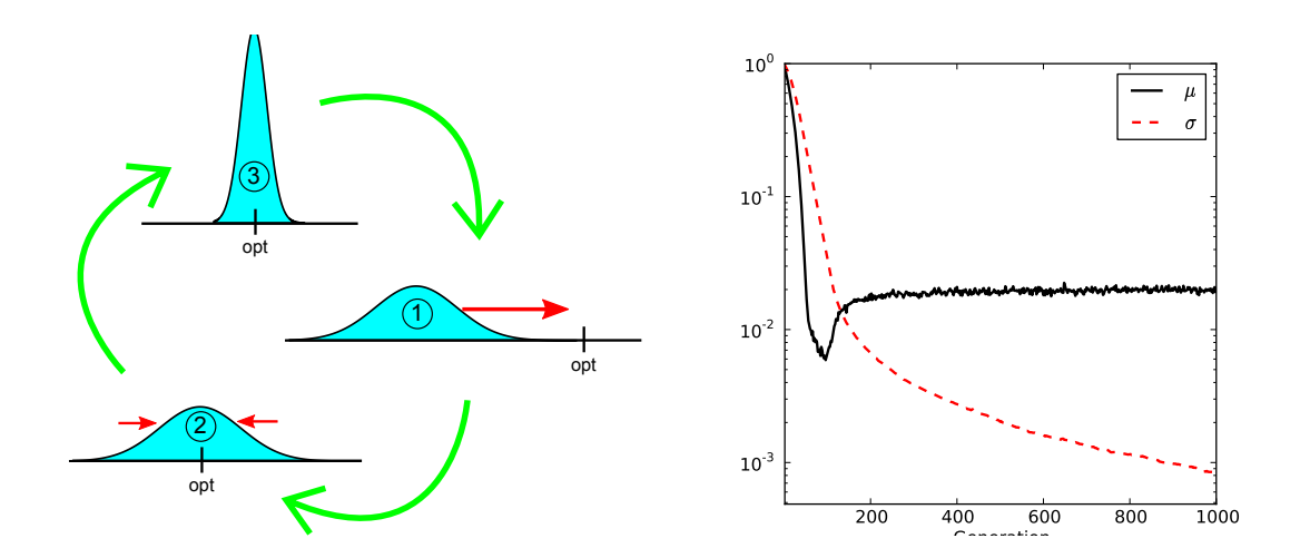
Figure 1: Left: Schematic illustration of how the search distribution adapts in the onedimensional case: from (1) to (2), µ is adjusted to make the distribution cover the optimum. From (2) to (3), σ is reduced to allow for a precise localization of the optimum. The step from (3) to (1) then is the problematic case, where a small σ induces a largely overshooting update, making the search start over again. Right: Progression of µ (black) and σ (red, dashed) when following the search gradient towards minimizing f(z) = z 2 , executing Algorithm 2. Plotted are median values over 1000 runs, with a small learning rate η = 0.01 and λ = 10, both of which mitigate the instability somewhat, but still show the failure to precisely locate the optimum (for which both µ and σ need to approach 0).

with ridges and plateaus, natural gradients are a more principled (and hyper-parameterfree) approach than, for example, the commonly used momentum heuristic.

The plain gradient ∇J simply follows the steepest ascent in the space of the actual parameters θ of the distribution. This means that for a given small step-size ε, following it will yield a new distribution with parameters chosen from the hypersphere of radius ǫ and center θ that maximizes J. In other words, the Euclidean distance in parameter space between subsequent distributions is fixed. Clearly, this makes the update dependent on the particular parameterization of the distribution, therefore a change of parameterization leads to different gradients and different updates. See also Figure 2 for an illustration of how this effectively renormalizes updates w.r.t. uncertainty.

The key idea of the natural gradient is to remove this dependence on the parameterization by relying on a more 'natural' measure of distance D(θ ′ ||θ) between probability distributions π (z|θ) and π (z|θ ′ ). One such natural distance measure between two probability distributions is the Kullback-Leibler divergence (Kullback and Leibler, 1951). The natural gradient can then be formalized as the solution to the constrained optimization

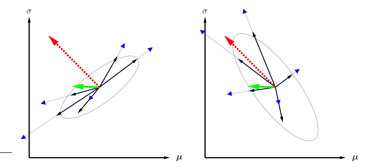
Figure 2: Illustration of plain versus natural gradient in parameter space. Consider two parameters, e.g. $\theta = (\mu, \sigma)$ , of the search distribution. In the plot on the left, the solid (black) arrows indicate the gradient samples $\nabla_{\theta} \log \pi(\mathbf{z} \mid \theta)$ , while the dotted (blue) arrows correspond to $f(\mathbf{z}) \cdot \nabla_{\theta} \log \pi(\mathbf{z} \mid \theta)$ , that is, the same gradient estimates, but scaled with fitness. Combining these, the bold (green) arrow indicates the (sampled) fitness gradient $\nabla_{\theta} J$ , while the bold dashed (red) arrow indicates the corresponding natural gradient $\tilde{\nabla}_{\theta} J$ .

Being random variables with expectation zero, the distribution of the black arrows is governed by their covariance, indicated by the gray ellipse. Notice that this covariance is a quantity in parameter space (where the $\theta$ reside), which is not to be confused with the covariance of the distribution in the search space (where the samples z reside).

In contrast, solid (black) arrows on the right represent $\tilde{\nabla}_{\theta} \log \pi(\mathbf{z} \mid \theta)$ , and dotted (blue) arrows indicate the natural gradient samples $f(\mathbf{z}) \cdot \tilde{\nabla}_{\theta} \log \pi(\mathbf{z} \mid \theta)$ , resulting in the natural gradient (dashed red).

The covariance of the solid arrows on the right hand side turns out to be the inverse of the covariance of the solid arrows on the left. This has the effect that when computing the natural gradient, directions with high variance (uncertainty) are penalized and thus shrunken, while components with low variance (high certainty) are boosted, since these components of the gradient samples deserve more trust. This makes the (dashed red) natural gradient a much more trustworthy update direction than the (green) plain gradient.

problem

$$\max_{\delta\theta} J(\theta + \delta\theta) \approx J(\theta) + \delta\theta^{\top} \nabla_{\theta} J,$$ s.t. $D(\theta + \delta\theta || \theta) = \varepsilon,$

where $J(\theta)$ is the expected fitness of equation (1), and $\varepsilon$ is a small increment size. Now, we have for $\delta\theta \to 0$ ,

$$D\left(\theta + \delta\theta || \theta\right) = \frac{1}{2} \delta\theta^{\top} \mathbf{F}\left(\theta\right) \delta\theta,$$

where

$$\mathbf{F} = \int \pi \left( \mathbf{z} | \theta \right) \nabla_{\theta} \log \pi \left( \mathbf{z} | \theta \right) \nabla_{\theta} \log \pi \left( \mathbf{z} | \theta \right)^{\top} d\mathbf{z},$$ $$= \mathbb{E} \left[ \nabla_{\theta} \log \pi \left( \mathbf{z} | \theta \right) \nabla_{\theta} \log \pi \left( \mathbf{z} | \theta \right)^{\top} \right]$$

is the Fisher information matrix of the given parametric family of search distributions. The solution to this can be found using a Lagrangian multiplier (Peters, 2007), yielding the necessary condition

$$\mathbf{F}\delta\theta = \beta\nabla_{\theta}J,\tag{5}$$

for some constant $\beta > 0$ . The direction of the natural gradient $\widetilde{\nabla}_{\theta} J$ is given by $\delta \theta$ thus defined. If F is invertible^{2}, the natural gradient amounts to

$$\widetilde{\nabla}_{\theta} J = \mathbf{F}^{-1} \nabla_{\theta} J(\theta).$$

The Fisher matrix can be estimated from samples, reusing the log-derivatives $\nabla_{\theta} \log \pi(\mathbf{z}|\theta)$ that we already computed for the gradient $\nabla_{\theta}J$ . Then, updating the parameters following the natural gradient instead of the steepest gradient leads us to the general formulation of NES, as shown in Algorithm 3.

3. Performance and Robustness Techniques

In the following we will present and introduce crucial techniques to improves NES's performance and robustness. Fitness shaping (Wierstra et al., 2008) is designed to make the algorithm invariant w.r.t. arbitrary yet order-preserving fitness transformations (section 3.1). Importance mixing (Sun et al., 2009b) is designed to recycle samples so as to reduce the number of required fitness evaluations, and is subsequently presented in section 3.2. Adaptation sampling, a novel technique for adjusting learning rates online, is introduced in section 3.3, and finally restart strategies, designed to improve success rates on multimodal problems, is presented in section 3.4.

3.1 Fitness Shaping

NES utilizes rank-based fitness shaping in order to render the algorithm invariant under monotonically increasing (i.e., rank preserving) transformations of the fitness function. For

^2. Care has to be taken because the Fisher matrix estimate may not be (numerically) invertible even if the exact Fisher matrix is.

Algorithm 3: Canonical Natural Evolution Strategies

input: f, \theta_{init}

repeat

for k = 1 ... \lambda do

draw sample \mathbf{z}_k \sim \pi(\cdot|\theta)
evaluate the fitness f(\mathbf{z}_k)
calculate log-derivatives \nabla_{\theta} \log \pi(\mathbf{z}_k|\theta)
end
\nabla_{\theta} J \leftarrow \frac{1}{\lambda} \sum_{k=1}^{\lambda} \nabla_{\theta} \log \pi(\mathbf{z}_k|\theta) \cdot f(\mathbf{z}_k)
\mathbf{F} \leftarrow \frac{1}{\lambda} \sum_{k=1}^{\lambda} \nabla_{\theta} \log \pi(\mathbf{z}_k|\theta) \nabla_{\theta} \log \pi(\mathbf{z}_k|\theta)^{\top}
\theta \leftarrow \theta + \eta \cdot \mathbf{F}^{-1} \nabla_{\theta} J
until stopping criterion is met

this purpose, the fitness of the population is transformed into a set of utility values $u_1 \ge \cdots \ge u_{\lambda}$ . Let $\mathbf{z}_i$ denote the $i^{th}$ best individual (the $i^{th}$ individual in the population, sorted by fitness, such that $\mathbf{z}_1$ is the best and $\mathbf{z}_{\lambda}$ the worst individual). Replacing fitness with utility, the gradient estimate of equation (2) becomes, with slight abuse of notation,

$$\nabla_{\theta} J(\theta) = \sum_{k=1}^{\lambda} u_k \, \nabla_{\theta} \log \pi(\mathbf{z}_k \,|\, \theta). \tag{6}$$

To avoid entangling the utility-weightings with the learning rate, we require that $\sum_{k=1}^{\lambda} |u_k| = 1$ .

The choice of utility function can in fact be seen as a free parameter of the algorithm. Throughout this paper we will use the following

$$u_k = \frac{\max\left(0, \log(\frac{\lambda}{2} + 1) - \log(i)\right)}{\sum_{j=1}^{\lambda} \max\left(0, \log(\frac{\lambda}{2} + 1) - \log(j)\right)} - \frac{1}{\lambda},$$

which is directly related to the one employed by CMA-ES (Hansen and Ostermeier, 2001), for ease of comparison. In our experience, however, this choice has not been crucial to performance, as long as it is monotonous and based on ranks instead of raw fitness (e.g., a function which simply increases linearly with rank).

In addition to robustness, these utility values provide us with an elegant formalism to describe the (1+1) hill-climber version of the algorithm within the same framework, by using different utility values, depending on success (see section 4.5 later in this paper).

3.2 Importance Mixing

In each batch, we evaluate $\lambda$ new samples generated from search distribution $\pi(\mathbf{z}|\theta)$ . However, since small updates ensure that the KL divergence between consecutive search distributions is generally small, most new samples will fall in the high density area of the previous

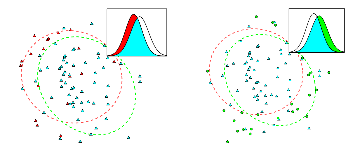
Figure 3: Illustration of importance mixing. Left: In the first step, old samples are eliminated (red triangles) according to (7), and the remaining samples (blue triangles) are reused. Right: In the second step, new samples (green circles) are generated according to (8).

search distribution $\pi(\mathbf{z}|\theta')$ . This leads to redundant fitness evaluations in that same area. We improve the efficiency with a new procedure called importance mixing, which aims at reusing fitness evaluations from the previous batch, while ensuring the updated batch conforms to the new search distribution.

Importance mixing works in two steps: In the first step, rejection sampling is performed on the previous batch, such that sample z is accepted with probability

$$\min \left\{ 1, (1 - \alpha) \frac{\pi \left( \mathbf{z} | \theta \right)}{\pi \left( \mathbf{z} | \theta' \right)} \right\}. \tag{7}$$

Here $\alpha \in [0, 1]$ is an algorithm hyperparameter called the minimal refresh rate. Let $\lambda_a$ be the number of samples accepted in the first step. In the second step, reverse rejection sampling is performed as follows: Generate samples from $\pi(\mathbf{z}|\theta)$ and accept $\mathbf{z}$ with probability

$$\max \left\{ \alpha, 1 - \frac{\pi \left( \mathbf{z} | \theta' \right)}{\pi \left( \mathbf{z} | \theta \right)} \right\} \tag{8}$$

until $\lambda - \lambda_a$ new samples are accepted. The $\lambda_a$ samples from the old batch and $\lambda - \lambda_a$ newly accepted samples together constitute the new batch. Figure 3 illustrates the procedure. Note that only the fitnesses of the newly accepted samples need to be evaluated. The advantage of using importance mixing is twofold: On the one hand, we reduce the number of fitness evaluations required in each batch, on the other hand, if we fix the number of newly evaluated fitnesses, then many more fitness evaluations can potentially be used to yield more reliable and accurate gradients.

The minimal refresh rate parameter $\alpha$ has two uses. First, it avoids too low an acceptance probability at the second step when $\pi\left(\mathbf{z}|\theta'\right)/\pi\left(\mathbf{z}|\theta\right)\simeq 1$ . And second, it permits specifying a lower bound on the expected proportion of newly evaluated samples $\rho=\mathbb{E}\left[\frac{\lambda-\lambda_a}{\lambda}\right]$ ,

namely ρ ≥ α, with the equality holding if and only if θ = θ ′ . In particular, if α = 1, all samples from the previous batch will be discarded, and if α = 0, ρ depends only on the distance between π (z|θ) and π (z|θ ′ ). Normally we set α to be a small positive number, e.g., in this paper we use α = 0.1 throughout.

It can be proven that the updated batch conforms to the search distribution π (z|θ). In the region where

$$(1 - \alpha) \frac{\pi(\mathbf{z}|\theta)}{\pi(\mathbf{z}|\theta')} \le 1,$$

the probability that a sample from previous batches appears in the new batch is

$$\pi\left(\mathbf{z}|\theta'\right)\cdot\left(1-\alpha\right)\frac{\pi\left(\mathbf{z}|\theta\right)}{\pi\left(\mathbf{z}|\theta'\right)}=\left(1-\alpha\right)\pi\left(\mathbf{z}|\theta\right).$$

The probability that a sample generated from the second step entering the batch is απ (z|θ), since

$$\max\left\{\alpha, 1 - \frac{\pi\left(\mathbf{z}|\theta'\right)}{\pi\left(\mathbf{z}|\theta\right)}\right\} = \alpha.$$

So the probability of a sample entering the batch is just p (z|θ) in that region. The same result holds also for the region where

$$(1-\alpha)\frac{\pi(\mathbf{z}|\theta)}{\pi(\mathbf{z}|\theta')} > 1.$$

When using importance mixing in the context of NES, this reduces the sensitivity to the hyperparameters, particularly the population size λ, as importance mixing implicitly adapts it to the situation by reusing some or many previously evaluated sample points.

3.3 Adaptation Sampling

To reduce the burden on determining appropriate hyper-parameters such as the learning rate, we develop a new self-adaptation or meta-learning technique (Schaul and Schmidhuber, 2010a), called adaptation sampling, that can automatically adapt the settings in a principled and economical way.

We model this situation as follows: Let π^θ be a distribution with hyper-parameter θ and ψ(z) a quality measure for each sample z ∼ πθ. Our goal is to adapt θ such as to maximize the quality ψ. A straightforward method to achieve this, henceforth dubbed adaptation sampling, is to evaluate the quality of the samples z ′ drawn from π^θ ′, where θ ′ ⁶⁼ ^θ is a slight variation of θ, and then perform hill-climbing: Continue with the new θ ′ if the quality of its samples is significantly better (according, e.g., to a Mann-Whitney U-test), and revert to θ otherwise. Note that this proceeding is similar to the NES algorithm itself, but applied at a meta-level to algorithm parameters instead of the search distribution. The goal of this adaptation is to maximize the pace of progress over time, which is slightly different from maximizing the fitness function itself.

Virtual adaptation sampling is a lightweight alternative to adaptation sampling that is particularly useful whenever evaluating ψ is expensive :

• do importance sampling on the existing samples $\mathbf{z}_i$ , according to $\pi_{\theta'}$ :

$$w_i' = \frac{\pi(\mathbf{z}|\theta')}{\pi(\mathbf{z}|\theta)}$$

(this is always well-defined, because $\mathbf{z} \sim \pi_{\theta} \Rightarrow \pi(\mathbf{z}|\theta) > 0$ ).

• compare $\{\psi(\mathbf{z}_i)\}$ with weights $\{w_i = 1, \forall i\}$ and $\{\psi' = \psi(\mathbf{z}_i), \forall i\}$ with weights $\{w'_i\}$ , using a weighted version of the Mann-Whitney test, as introduced in Appendix A.

Beyond determining whether $\theta$ or $\theta'$ is better, choosing a non-trivial confidence level $\rho$ allows us to avoid parameter drift, as $\theta$ is only updated if the improvement is significant enough.

There is one caveat, however: the rate of parameter change needs to be adjusted such that the two resulting distributions are not too similar (otherwise the difference won't be statistically significant), but also not too different, (otherwise the weights w' will be too small and again the test will be inconclusive).

If, however, we explicitly desire large adaptation steps on $\theta$ , we have the possibility of interpolating between adaptation sampling and virtual adaptation sampling by drawing a few new samples from the distribution $\pi_{\theta'}$ (each assigned weight 1), where it is overlapping least with $\pi_{\theta}$ . The best way of achieving this is importance mixing, as introduced in Section 3.2, uses jointly with the reweighted existing samples.

For NES algorithms, the most important parameter to be adapted by adaptation sampling is the learning rate $\eta$ , starting with a conservative guess. This is because half-way into the search, after a local attractor has been singled out, it may well pay off to increase the learning rate in order to more quickly converge to it.

In order to produce variations $\eta'$ which can be judged using the above-mentioned Utest, we propose a procedure similar in spirit to Rprop-updates (Riedmiller and Braun, 1993; Igel and Husken, 2003), where the learning rates are either increased or decreased by a multiplicative constant whenever there is evidence that such a change will lead to better samples.

More concretely, when using adaptation sampling for NES we test for an improvement with the hypothetical distribution $\theta'$ generated with $\eta' = 1.5\eta$ . Each time the statistical test is successful with a confidence of at least $\rho = \frac{1}{2} - \frac{1}{3(d+1)}$ (this value was determined empirically) we increase the learning rate by a factor of $c^+ = 1.1$ , up to at most $\eta = 1$ . Otherwise we bring it closer to its initial value: $\eta \leftarrow 0.9\eta + 0.1\eta_{init}$ .

Figure 4 illustrates the effect of the virtual adaptation sampling strategy on two different 10-dimensional unimodal benchmark functions, the Sphere function $f_1$ and the Rosenbrock function $f_8$ (see section 6.2 for details). We find that, indeed, adaptation sampling boosts the learning rates to the appropriate high values when quick progress can be made (in the presence of an approximately quadratic optimum), but keeps them at carefully low values otherwise.

3.4 Restart Strategies

A simple but widespread method for mitigating the risk of finding only local optima in a strongly multi-modal scenario is to restart the optimization algorithm a number of times

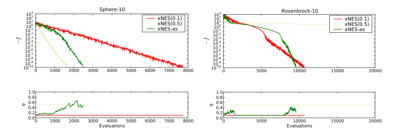
Figure 4: Illustration of the effect of adaptation sampling. We show the increase in fitness during a NES run (above) and the corresponding learning rates (below) on two setups: 10-dimensional sphere function (left), and 10-dimensional Rosenbrock function (right). Plotted are three variants of xNES (algorithm 4): fixed default learning rate of $\eta=0.1$ (dashed, red) fixed large learning rate of $\eta=0.5$ (dotted, yellow), and an adaptive learning rate starting at $\eta=0.1$ (green). We see that for the (simple) Sphere function, it is advantageous to use a large learning rate, and adaptation sampling automatically finds that one. However, using the overly greedy updates of a large learning rate fails on harder problems (right). Here adaptation sampling really shines: it boosts the learning rate in the initial phase (entering the Rosenbrock valley), then quickly reduces it while the search needs to carefully navigate the bottom of the valley, and boosts it again at the end when it has located the optimum and merely needs to zoom in precisely.

with different initializations, or just with a different random seed. This is even more useful in the presence of parallel processing resources, in which case multiple runs are executed simultaneously.

In practice, where the parallel capacity is limited, we need to decide when to stop or suspend an ongoing optimization run and start or resume another one. In this section we provide one such restart strategy that takes those decisions. Inspired by recent work on practical universal search (Schaul and Schmidhuber, 2010b), this results in an effective use of resources independently of the problem.

The strategy consists in reserving a fixed fraction p of the total time for the first run, and then subdividing the remaining time 1-p in the same way, recursively (i.e. $p(1-p)^{i-1}$ for the $i^{th}$ run). The recursive decomposition of the time budget stops when the assigned time-slice becomes smaller than the overhead of swapping out different runs. In this way, the number of runs with different seeds remains finite, but increases over time, as needed. Figure 5 illustrates the effect of the restart strategy, for different values of p, on the example of a multi-modal benchmark function $f_{18}$ (see section 6.2 for details), where most runs get caught in local optima. Whenever used in the rest of the paper, the fraction is $p = \frac{1}{5}$ .

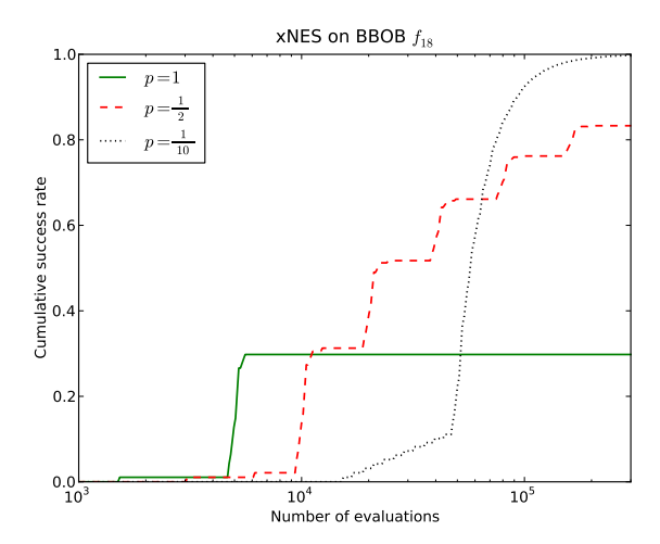
Figure 5: Illustrating the effect of different restart strategies. Plotted is the cumulative empirical success probability, as a function of the total number of evaluations used. Using no restarts, corresponding to p=1 (green) is initially faster but unreliable, whereas $p=\frac{1}{10}$ (dotted black) reliably finds the optimum within 300000 evaluations, but at the cost of slowing down success for all runs by a factor 10. In-between these extremes, $p=\frac{1}{2}$ (broken line, red) trades off slowdown and reliability.

Let s(t) be the success probability of the underlying search algorithm at time t. Here, time is measured by the number of generations or fitness evaluations. Accordingly, let $S_p(t)$ be the boosted success probability of the restart scheme with parameter p. Approximately, that is, assuming continuous time, the probabilities are connected by the formula

$$S_p(t) = 1 - \prod_{i=1}^{\infty} \left[ 1 - s(p(1-p)^{i-1}t) \right].$$

Two qualitative properties of the restart strategy can be deduced from this formula, even if in discrete time the sum is finite $(i \leq \log_2(t))$ , and the times $p(1-p)^{i-1}t$ need to be rounded:

If there exists $t_0$ such that $s(t_0) > 0$ then $\lim_{t \to \infty} S_p(t) = 1$ for all $p \in (0,1)$ .
For sufficiently small t, we have $S_p(t) \leq s_p(t)$ .

This captures the expected effect that the restart strategy results in an initial slowdown, but eventually solves the problem reliably.

4. Techniques for Multinormal Distributions

In this section we will describe two crucial techniques to enhance performance of the NES algorithm as applied to multinormal distributions. First, the method of exponential parameterization is introduced, guaranteeing that the covariance matrix stays positive-definite.

Second, a novel method for changing the coordinate system into a "natural" one is laid out, making the algorithm computationally efficient.

4.1 Using Exponential Parameterization

Gradient steps on the covariance matrix $\Sigma$ result in a number of technical problems. When updating $\Sigma$ directly with the gradient step $\nabla_{\Sigma} J$ , we have to ensure that $\Sigma + \eta \nabla_{\Sigma} J$ remains a valid, positive definite covariance matrix. This is not guaranteed a priori, because the (natural) gradient $\nabla_{\Sigma} J$ may be any symmetric matrix. If we instead update a factor $\mathbf{A}$ of $\Sigma$ , it is at least ensured that $\mathbf{A}^{\top} \mathbf{A}$ is symmetric and positive semi-definite. But when shrinking an eigenvalue of $\mathbf{A}$ it may happen that the gradient step swaps the sign of the eigenvalue, resulting in undesired oscillations.

An elegant way to fix these problems is to represent the covariance matrix using the exponential map for symmetric matrices (see e.g., Glasmachers and Igel, 2005 for a related approach). Let

$$\mathcal{S}_d := \left\{ \mathbf{M} \in \mathbb{R}^{d imes d} \,\middle|\, \mathbf{M}^ op = \mathbf{M} ight\}$$

and

$$\mathcal{P}_d := \left\{ \mathbf{M} \in \mathcal{S}_d \,\middle|\, \mathbf{v}^\top \mathbf{M} \mathbf{v} > 0 \text{ for all } \mathbf{v} \in \mathbb{R}^d \setminus \{0\} \right\}$$

denote the vector space of symmetric and the (cone) manifold of symmetric positive definite matrices, respectively. Then the exponential map

$$\exp: \mathcal{S}_d \to \mathcal{P}_d , \qquad \mathbf{M} \mapsto \sum_{n=0}^{\infty} \frac{\mathbf{M}^n}{n!} \tag{9} $$

is a diffeomorphism: The map is bijective, and both exp as well as its inverse map $\log : \mathcal{P}_d \to \mathcal{S}_d$ are smooth. The mapping can be computed in cubic time, for example by decomposing the matrix $\mathbf{M} = \mathbf{U}\mathbf{D}\mathbf{U}^{\top}$ into orthogonal $\mathbf{U}$ (eigen-vectors) and diagonal $\mathbf{D}$ (eigen-values), taking the exponential of $\mathbf{D}$ (which amounts to taking the element-wise exponentials of the diagonal entries), and composing everything back^{3} as $\exp(\mathbf{M}) = \mathbf{U} \exp(\mathbf{D})\mathbf{U}^{\top}$ .

Thus, we can represent the covariance matrix $\Sigma \in \mathcal{P}_d$ as $\exp(\mathbf{M})$ with $\mathbf{M} \in \mathcal{S}_d$ . The resulting gradient update for $\mathbf{M}$ has two important properties: First, because $\mathcal{S}_d$ is a vector space, any update automatically corresponds to a valid covariance matrix.⁴ Second, the update of $\mathbf{M}$ makes the gradient invariant w.r.t. linear transformations of the search space $\mathbb{R}^d$ . This follows from an information geometric perspective, viewing $\mathcal{P}_d$ as the Riemannian parameter manifold equipped with the Fisher information metric. The invariance property is a direct consequence of the Cartan-Hadamard theorem (Cartan, 1928). See also Figure 6 for an illustration.

However, the exponential parameterization considerably complicates the computation of the Fisher information matrix $\mathbf{F}$ , which now involves partial derivatives of the matrix exponential (9). This can be done in cubic time per partial derivative according

^3. The same computation works for the logarithm, and thus also for powers $\mathcal{P}_d \to \mathcal{P}_d$ , $\mathbf{M} \mapsto \mathbf{M}^c = \exp(c \cdot \log(\mathbf{M}))$ for all $c \in \mathbb{R}$ , for example for the (unique) square root (c = 1/2).

^4. The tangent bundle $T\mathcal{P}_d$ of the manifold $\mathcal{P}_d$ is isomorphic to $\mathcal{P}_d \times \mathcal{S}_d$ and globally trivial. Thus, arbitrarily large gradient steps are meaningful in this representation.

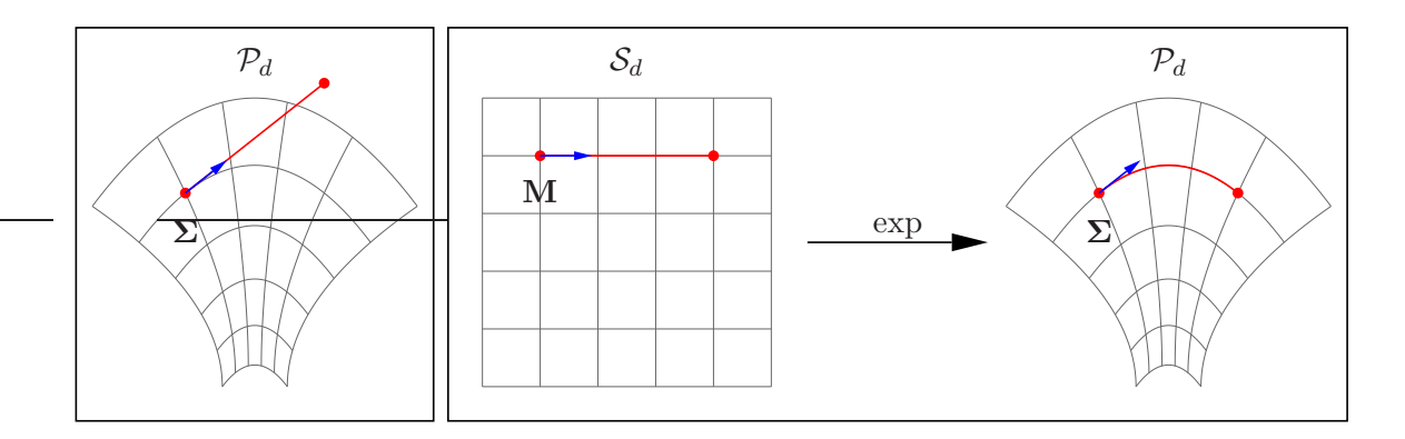
Figure 6: Left: updating a covariance matrix $\Sigma$ directly can end up outside the manifold of symmetric positive-definite matrices $\mathcal{P}_d$ . Right: first performing the update on $\mathbf{M} = \frac{1}{2} \log(\Sigma)$ in $\mathcal{S}_d$ and then mapping back the result into the original space $\mathcal{P}_d$ using the exponential map is both safe (guaranteed to stay in the manifold) and straight (the update follows a geodesic).

to (Najfeld and Havel, 1994), resulting in an unacceptable complexity of $\mathcal{O}(d^7)$ for the computation of the Fisher matrix.

4.2 Using Natural Coordinates

In this section we describe a technique that allows us to avoid the computation of the Fisher information matrix altogether, for some specific but common classes of distributions. The idea is to iteratively change the coordinate system in such a way that it becomes possible to follow the natural gradient without any costly inverses of the Fisher matrix (actually, without even constructing it explicitly). We introduce the technique for the simplest case of multinormal search distributions, and in section 5.2, we generalize it to the whole class of distributions that they are applicable to (namely, rotationally-symmetric distributions).

Instead of using the 'global' coordinates $\Sigma = \exp(\mathbf{M})$ for the covariance matrix, we linearly transform the coordinate system in each iteration to a coordinate system in which the current search distribution is the standard normal distribution with zero mean and unit covariance. Let the current search distribution be given by $(\boldsymbol{\mu}, \mathbf{A}) \in \mathbb{R}^d \times \mathcal{P}_d$ with $\mathbf{A}^{\top} \mathbf{A} = \Sigma$ . We use the tangent space $T_{(\boldsymbol{\mu}, \mathbf{A})}(\mathbb{R}^d \times \mathcal{P}_d)$ of the parameter manifold $\mathbb{R}^d \times \mathcal{P}_d$ , which is isomorphic to the vector space $\mathbb{R}^d \times \mathcal{S}_d$ , to represent the updated search distribution as

$$(\boldsymbol{\delta}, \mathbf{M}) \mapsto (\boldsymbol{\mu}_{\text{new}}, \mathbf{A}_{\text{new}}) = \left(\boldsymbol{\mu} + \mathbf{A}^{\top} \boldsymbol{\delta}, \mathbf{A} \exp\left(\frac{1}{2}\mathbf{M}\right)\right). \tag{10} $$

This coordinate system is natural in the sense that the Fisher matrix w.r.t. an orthonormal basis of $(\boldsymbol{\delta}, \mathbf{M})$ is the identity matrix. The current search distribution $\mathcal{N}(\boldsymbol{\mu}, \mathbf{A}^{\top} \mathbf{A})$ is encoded as

$$\pi(\mathbf{z}|\boldsymbol{\delta}, \mathbf{M}) = \mathcal{N}\left(\boldsymbol{\mu} + \mathbf{A}^{\top}\boldsymbol{\delta}, \ \mathbf{A}^{\top}\exp(\mathbf{M})\mathbf{A}\right),$$

where at each step we change the coordinates such that $(\boldsymbol{\delta}, \mathbf{M}) = (0, 0)$ . In this case, it is guaranteed that for the variables $(\boldsymbol{\delta}, \mathbf{M})$ the plain gradient and the natural gradient coincide $(\mathbf{F} = \mathbb{I})$ . Consequently the computation of the natural gradient costs $\mathcal{O}(d^3)$ operations.

In the new coordinate system we produce standard normal samples $\mathbf{s} \sim \mathcal{N}(0, \mathbb{I})$ which are then mapped back into the original coordinates $\mathbf{z} = \boldsymbol{\mu} + \mathbf{A}^{\top} \cdot \mathbf{s}$ . The log-density becomes

$$\log \pi(\mathbf{z} \mid \boldsymbol{\delta}, \mathbf{M}) = -\frac{d}{2} \log(2\pi) - \log \left( \det(\mathbf{A}) \right) - \frac{1}{2} \operatorname{tr}(\mathbf{M})$$ $$-\frac{1}{2} \left\| \exp \left( -\frac{1}{2} \mathbf{M} \right) \mathbf{A}^{-\top} \cdot (\mathbf{z} - (\boldsymbol{\mu} + \mathbf{A}^{\top} \boldsymbol{\delta})) \right\|^{2},$$

and thus the log-derivatives (at $\delta = 0$ , $\mathbf{M} = 0$ ) take the following, surprisingly simple forms:

$$\nabla_{\boldsymbol{\delta}}|_{\boldsymbol{\delta}=0} \log \pi(\mathbf{z} \mid \mathbf{M} = 0, \boldsymbol{\delta}) = \nabla_{\boldsymbol{\delta}}|_{\boldsymbol{\delta}=0} \left[ -\frac{1}{2} \left\| \mathbf{A}^{-\top} \cdot (\mathbf{z} - (\boldsymbol{\mu} + \mathbf{A}^{\top} \boldsymbol{\delta})) \right\|^{2} \right]$$

$$= -\frac{1}{2} \left[ -2 \cdot \mathbf{A}^{-\top} \mathbf{A}^{\top} \cdot \mathbf{A}^{-\top} \cdot (\mathbf{z} - (\boldsymbol{\mu} + \mathbf{A}^{\top} \boldsymbol{\delta})) \right] \Big|_{\boldsymbol{\delta}=0}$$

$$= \mathbf{A}^{-\top} (\mathbf{z} - \boldsymbol{\mu})$$

$$= \mathbf{s}$$ \tag{11} $$$$ $$\nabla_{\mathbf{M}}|{\mathbf{M}=0} \log \pi(\mathbf{z} \mid \boldsymbol{\delta} = 0, \mathbf{M}) = -\frac{1}{2} \nabla{\mathbf{M}}|{\mathbf{M}=0} \left[ \operatorname{tr}(\mathbf{M}) + \left| \exp\left(-\frac{1}{2}\mathbf{M}\right) \mathbf{A}^{-\top} (\mathbf{z} - \boldsymbol{\mu}) \right|^{2} \right]$$ $$= -\frac{1}{2} \left[ \mathbb{I} + 2 \cdot \left( -\frac{1}{2} \right) \cdot \left[ \mathbf{A}^{-\top} (\mathbf{z} - \boldsymbol{\mu}) \right] \cdot \exp\left( -\frac{1}{2}\mathbf{M} \right) \cdot \left[ \mathbf{A}^{-\top} (\mathbf{z} - \boldsymbol{\mu}) \right]^{\top} \right] \Big|{\mathbf{M}=0}$$ $$= -\frac{1}{2} \left[ \mathbb{I} - \left[ \mathbf{A}^{-\top} (\mathbf{z} - \boldsymbol{\mu}) \right] \cdot \mathbb{I} \cdot \left[ \mathbf{A}^{-\top} (\mathbf{z} - \boldsymbol{\mu}) \right]^{\top} \right]$$ $$= \frac{1}{2} (\mathbf{s}\mathbf{s}^{\top} - \mathbb{I})$$ \tag{12} $$$$ These results give us the updates in the natural coordinate system $$\nabla_{\delta} J = \sum_{k=1}^{\lambda} f(\mathbf{z}k) \cdot \mathbf{s}_k \tag{13}$$ $$\nabla{\mathbf{M}} J = \sum_{k=1}^{\lambda} f(\mathbf{z}k) \cdot (\mathbf{s}_k \mathbf{s}_k^{\top} - \mathbb{I}) \tag{14} $$ which are then mapped back onto $(\mu, \mathbf{A})$ using equation (10): $$\begin{split} \boldsymbol{\mu}{\text{new}} \leftarrow \boldsymbol{\mu} + \mathbf{A}^{\top} \boldsymbol{\delta} &= \boldsymbol{\mu} + \eta \mathbf{A}^{\top} \nabla_{\boldsymbol{\delta}} J \ &= \boldsymbol{\mu} + \eta \mathbf{A}^{\top} \left( \frac{1}{\lambda} \sum_{k=1}^{\lambda} \nabla_{\boldsymbol{\delta}} \log \pi \left( \mathbf{z}{k} | \boldsymbol{\theta} \right) \cdot f(\mathbf{z}{k}) \right) \ &= \boldsymbol{\mu} + \frac{\eta}{\lambda} \mathbf{A}^{\top} \left( \sum_{k=1}^{\lambda} f(\mathbf{z}{k}) \cdot \mathbf{s}{k} \right) \ \mathbf{A}{\text{new}} \leftarrow \mathbf{A} \cdot \exp \left( \frac{1}{2} \mathbf{M} \right) &= \mathbf{A} \cdot \exp \left( \eta \frac{1}{2} \nabla{\mathbf{M}} J \right) \ &= \mathbf{A} \cdot \exp \left( \frac{\eta}{2} \cdot \frac{1}{\lambda} \sum_{k=1}^{\lambda} \nabla_{\mathbf{M}} \log \pi \left( \mathbf{z}{k} | \boldsymbol{\theta} \right) \cdot f(\mathbf{z}{k}) \right) \ &= \mathbf{A} \cdot \exp \left( \frac{\eta}{4\lambda} \sum_{k=1}^{\lambda} f(\mathbf{z}{k}) \cdot (\mathbf{s}{k} \mathbf{s}{k}^{\top} - \mathbb{I}) \right) \end{split}$$ #### 4.3 Orthogonal Decomposition of Multinormal Parameter Space We decompose the parameter vector space $(\boldsymbol{\delta}, \mathbf{M}) \in \mathbb{R}^d \times \mathcal{S}_d$ into the product $$\mathbb{R}^d \times \mathcal{S}_d = \underbrace{\mathbb{R}^d}{(\delta)} \times \underbrace{\mathcal{S}d^{\parallel}}{(\sigma)} \times \underbrace{\mathcal{S}d^{\perp}}{(\mathbf{B})} , \qquad (15)$$ of orthogonal subspaces. The one-dimensional space $\mathcal{S}_d^{\parallel} = \{\lambda \cdot \mathbb{I} \mid \lambda \in \mathbb{R}\}$ is spanned by the identity matrix $\mathbb{I}$ , and $\mathcal{S}_d^{\perp} = \{\mathbf{M} \in \mathcal{S}_d \mid \operatorname{tr}(\mathbf{M}) = 0\}$ denotes its orthogonal complement in $\mathcal{S}_d$ . The different components have roles with clear interpretations: The $(\delta)$ -component $\nabla_{\delta}J$ describes the update of the center of the search distribution, the $(\sigma)$ -component with value $\nabla_{\sigma}J \cdot \mathbb{I}$ for $\nabla_{\sigma}J = \operatorname{tr}(\nabla_{\mathbf{M}}J)/d$ has the role of a step size update, which becomes clear from the identity $\det(\exp(\mathbf{M})) = \exp(\operatorname{tr}(\mathbf{M}))$ , and the $(\mathbf{B})$ -component $\nabla_{\mathbf{B}}J = \nabla_{\mathbf{M}}J - \nabla_{\sigma}J$ describes the update of the transformation matrix, normalized to unit determinant, which can thus be attributed to the shape of the search distribution. This decomposition is canonical in being the finest decomposition such that updates of its components result in invariance of the search algorithm under linear transformations of the search space. On these subspaces we introduce independent learning rates $\eta_{\delta}$ , $\eta_{\sigma}$ , and $\eta_{\mathbf{B}}$ , respectively. For simplicity we also split the transformation matrix $\mathbf{A} = \sigma \cdot \mathbf{B}$ into the step size $\sigma \in \mathbb{R}^+$ and the normalized transformation matrix $\mathbf{B}$ with $\det(\mathbf{B}) = 1$ . Then the resulting update is $$\mu_{\text{new}} = \mu + \eta_{\delta} \cdot \nabla_{\delta} J = \mu + \eta_{\delta} \cdot \sum_{k=1}^{\lambda} f(\mathbf{z}k) \cdot \mathbf{s}_k \tag{16} $$ $$\sigma{\text{new}} = \sigma \cdot \exp\left(\frac{\eta_{\sigma}}{2} \cdot \nabla_{\sigma}\right) = \sigma \cdot \exp\left(\frac{\eta_{\sigma}}{2} \cdot \frac{\operatorname{tr}(\nabla_{\mathbf{M}}J)}{d}\right) \tag{17} $$ $$\mathbf{B}{\text{new}} = \mathbf{B} \cdot \exp\left(\frac{\eta{\mathbf{B}}}{2} \cdot \nabla_{\mathbf{B}} J\right) = \mathbf{B} \cdot \exp\left(\frac{\eta_{\mathbf{B}}}{2} \cdot \left(\nabla_{\mathbf{M}} J - \frac{\operatorname{tr}(\nabla_{\mathbf{M}} J)}{d} \cdot \mathbb{I}\right)\right), \tag{18}$$ with $\nabla_{\mathbf{M}}J$ from equation (14). In case of $\eta_{\sigma} = \eta_{\mathbf{B}}$ , in this case referred to as $\eta_{\mathbf{A}}$ , the updates (17) and (18) simplify to $$\mathbf{A}{\text{new}} = \mathbf{A} \cdot \exp\left(\frac{\eta{\mathbf{A}}}{2} \cdot \nabla_{\mathbf{M}}\right)$$ $$= \mathbf{A} \cdot \exp\left(\frac{\eta_{\mathbf{A}}}{2} \cdot \sum_{k=1}^{\lambda} f(\mathbf{z}{k}) \cdot (\mathbf{s}{k} \mathbf{s}_{k}^{\top} - \mathbb{I})\right). \tag{19} $$

The resulting algorithm is called exponential NES (xNES), and shown in Algorithm 4. We also give the pseudocode for its hill-climber variant (see also section 4.5).

Updating the search distribution in the natural coordinate system is an alternative to the exponential parameterization (section 4.1) for making the algorithm invariant under linear transformations of the search space, which is then achieved in a direct and constructive way.

Algorithm 4: Exponential Natural Evolution Strategies (xNES), for multinormal distributions

input: f, \mu_{init}, \Sigma_{init} = \mathbf{A}^{\top} \mathbf{A}

initialize \sigma \leftarrow \sqrt[d]{\det(\mathbf{A})|}
\mathbf{B} \leftarrow \mathbf{A}/\sigma

repeat

for k = 1 \dots \lambda do

draw sample \mathbf{s}_k \sim \mathcal{N}(0, \mathbb{I})
\mathbf{z}_k \leftarrow \boldsymbol{\mu} + \sigma \mathbf{B}^{\top} \mathbf{s}_k
evaluate the fitness f(\mathbf{z}_k)
end
sort \{(\mathbf{s}_k, \mathbf{z}_k)\} with respect to f(\mathbf{z}_k) and compute utilities u_k

compute gradients \nabla_{\delta} J \leftarrow \sum_{k=1}^{\lambda} u_k \cdot \mathbf{s}_k \quad \nabla_{\mathbf{M}} J \leftarrow \sum_{k=1}^{\lambda} u_k \cdot (\mathbf{s}_k \mathbf{s}_k^{\top} - \mathbb{I})
\nabla_{\sigma} J \leftarrow \operatorname{tr}(\nabla_{\mathbf{M}} J)/d \quad \nabla_{\mathbf{B}} J \leftarrow \nabla_{\mathbf{M}} J - \nabla_{\sigma} J \cdot \mathbb{I}

\mu \leftarrow \mu + \eta_{\delta} \cdot \sigma \mathbf{B} \cdot \nabla_{\delta} J
update parameters \sigma \leftarrow \sigma \cdot \exp(\eta_{\sigma}/2 \cdot \nabla_{\sigma} J)
\mathbf{B} \leftarrow \mathbf{B} \cdot \exp(\eta_{\mathbf{B}}/2 \cdot \nabla_{\mathbf{B}} J)
until stopping criterion is met

4.4 Connection to CMA-ES.

It has been noticed independently by (Glasmachers et al., 2010a) and shortly afterwards by (Akimoto et al., 2010) that the natural gradient updates of xNES and the strategy updates of the CMA-ES algorithm (Hansen and Ostermeier, 2001) are closely connected. However, since xNES does not feature evolution paths, this connection is restricted to the so-called rank- $\mu$ -update (in the terminology of this study, rank- $\lambda$ -update) of CMA-ES.

Algorithm 5: (1+1)-xNES

input: f, \mu_{init}, \Sigma_{init} = \mathbf{A}^{\top} \mathbf{A}
f_{max} \leftarrow -\infty
repeat
\begin{vmatrix}
\text{draw sample } \mathbf{s} \sim \mathcal{N}(0, \mathbb{I}) \\
\text{evaluate the fitness } f(\mathbf{z} = \mathbf{A}^{\top} \mathbf{s} + \boldsymbol{\mu}) \\
\text{calculate log-derivatives } \nabla_{\mathbf{M}} \log \pi (\mathbf{z} | \boldsymbol{\theta}) = \frac{1}{2} (\mathbf{s} \mathbf{s}^{\top} - \mathbb{I}) \\
(\mathbf{z}_{1}, \mathbf{z}_{2}) \leftarrow (\boldsymbol{\mu}, \mathbf{z}) \\
\text{if } f_{max} < f(\mathbf{z}) \text{ then} \\
| f_{max} \leftarrow f(\mathbf{z}) \\
\mathbf{u} \leftarrow (-4, 1) \\
| \text{update mean } \boldsymbol{\mu} \leftarrow \mathbf{z} \\
\text{else} \\
| \mathbf{u} \leftarrow (\frac{4}{5}, 0) \\
\text{end} \\
\nabla_{\mathbf{M}} J \leftarrow \frac{1}{2} \sum_{k=1}^{2} \nabla_{\mathbf{M}} \log \pi (\mathbf{z}_{k} | \boldsymbol{\theta}) \cdot u_{k} = -\frac{u_{1}}{2} \mathbb{I} + \frac{u_{2}}{4} (\mathbf{s} \mathbf{s}^{\top} - \mathbb{I}) \\
\mathbf{A} \leftarrow \mathbf{A} \cdot \exp \left(\frac{1}{2} \eta \nabla_{\mathbf{M}} J\right) \\
\text{until stopping criterion is met}

First of all observe that xNES and CMA-ES share the same invariance properties. But more interestingly, although derived from different heuristics, their updates turn out to be nearly equivalent. A closer investigation of this equivalence promises synergies and new perspectives on the working principles of both algorithms. In particular, this insight shows that CMA-ES can be explained as a natural gradient algorithm, which may allow for a more thorough analysis of its updates, and xNES can profit from CMA-ES's mature settings of algorithms parameters, such as search space dimension-dependent population sizes, learning rates and utility values.

Both xNES and CMA-ES parameterize the search distribution with three functionally different parameters for mean, scale, and shape of the distribution. xNES uses the parameters $\mu$ , $\sigma$ , and $\mathbf{B}$ , while the covariance matrix is represented as $\sigma^2 \cdot \mathbf{C}$ in CMA-ES, where $\mathbf{C}$ can by any positive definite symmetric matrix. Thus, the representation of the scale of the search distribution is shared among $\sigma$ and $\mathbf{C}$ in CMA-ES, and the role of the additional parameter $\sigma$ is to allow for an adaptation of the step size on a faster time scale than the full covariance update. In contrast, the NES updates of scale and shape parameters $\sigma$ and $\mathbf{B}$ are properly decoupled.

Let us start with the updates of the center parameter $\mu$ . The update (16) is very similar to the update of the center of the search distribution in CMA-ES, see (Hansen and Ostermeier, 2001). The utility function exactly takes the role of the weights in CMA-ES, which assumes a fixed learning rate of one.

For the covariance matrix, the situation is more complicated. From equation (19) we deduce the update rule

$$\begin{split} \boldsymbol{\Sigma}_{\text{new}} = & (\mathbf{A}_{\text{new}})^{\top} \cdot \mathbf{A}_{\text{new}} \\ = & \mathbf{A}^{\top} \cdot \exp \left( \eta_{\boldsymbol{\Sigma}} \cdot \sum_{k=1}^{\lambda} u_k \left( \mathbf{s}_k \mathbf{s}_k^{\top} - \mathbb{I} \right) \right) \cdot \mathbf{A} \end{split}$$

for the covariance matrix, with learning rate $\eta_{\Sigma} = \eta_{\mathbf{A}}$ . This term is closely connected to the exponential parameterization of the natural coordinates in xNES, while CMA-ES is formulated in global linear coordinates. The connection of these updates can be shown either by applying the xNES update directly to the natural coordinates without the exponential parameterization, or by approximating the exponential map by its first order Taylor expansion. (Akimoto et al., 2010) established the same connection directly in coordinates based on the Cholesky decomposition of $\Sigma$ , see (Sun et al., 2009a,b). The arguably simplest derivation of the equivalence relies on the invariance of the natural gradient under coordinate transformations, which allows us to perform the computation, w.l.o.g., in natural coordinates. We use the first order Taylor approximation of exp to obtain

$$\exp\left(\eta_{\Sigma} \cdot \sum_{k=1}^{\lambda} u_k \left(\mathbf{s}_k \mathbf{s}_k^{\top} - \mathbb{I}\right)\right) \approx \mathbb{I} + \eta_{\Sigma} \cdot \sum_{k=1}^{\lambda} u_k \left(\mathbf{s}_k \mathbf{s}_k^{\top} - \mathbb{I}\right) ,$$

so the first order approximate update yields

$$\mathbf{\Sigma}'_{new} = \mathbf{A}^{\top} \cdot \left( \mathbb{I} + \eta_{\mathbf{\Sigma}} \cdot \sum_{k=1}^{\lambda} u_k \left( \mathbf{s}_k \mathbf{s}_k^{\top} - \mathbb{I} \right) \right) \cdot \mathbf{A}$$

$$= (1 - U \cdot \eta_{\mathbf{\Sigma}}) \cdot \mathbf{A}^{\top} \mathbf{A} + \eta_{\mathbf{\Sigma}} \cdot \sum_{k=1}^{\lambda} u_k \left( \mathbf{A}^{\top} \mathbf{s}_k \right) \left( \mathbf{A}^{\top} \mathbf{s}_k \right)^{\top}$$

$$= (1 - U \cdot \eta_{\mathbf{\Sigma}}) \cdot \mathbf{\Sigma} + \eta_{\mathbf{\Sigma}} \cdot \sum_{k=1}^{\lambda} u_k \left( \mathbf{z}_k - \boldsymbol{\mu} \right) \left( \mathbf{z}_k - \boldsymbol{\mu} \right)^{\top}$$

with $U = \sum_{k=1}^{\lambda} u_k$ , from which the connection to the CMA-ES rank- $\mu$ -update is obvious (see Hansen and Ostermeier, 2001).

Finally, the updates of the global step size parameter $\sigma$ turn out to be identical in xNES and CMA-ES without evolution paths.

Having highlighted the similarities, let us have a closer look at the differences between xNES and CMA-ES, which are mostly two aspects. CMA-ES uses the well-established technique of evolution paths to smoothen out random effects over multiple generations. This technique is particularly valuable when working with minimal population sizes, which is the default for both algorithms. Thus, evolution paths are expected to improve stability; further interpretations have been provided by (Hansen and Ostermeier, 2001). However, the presence of evolution paths has the conceptual disadvantage that the state of the CMA-ES algorithms is not completely described by its search distribution. The other difference between xNES and CMA-ES is the exponential parameterization of the updates in xNES,

which results in a multiplicative update equation for the covariance matrix, in contrast to the additive update of CMA-ES. We argue that just like for the global step size $\sigma$ , the multiplicative update of the covariance matrix is natural.

A valuable perspective offered by the natural gradient updates in xNES is the derivation of the updates of the center $\mu$ , the step size $\sigma$ , and the normalized transformation matrix B, all from the same principle of natural gradient ascent. In contrast, the updates applied in CMA-ES result from different heuristics for each parameter. Hence, it is even more surprising that the two algorithms are closely connected. This connection provides a post-hoc justification of the various heuristics employed by CMA-ES, and it highlights the consistency of the intuition behind these heuristics.

4.5 Elitism

The principle of the NES algorithm is to follow the natural gradient of expected fitness. This requires sampling the fitness gradient. Naturally, this amounts to what, within the realm of evolution strategies, is generally referred to as "comma-selection", that is, updating the search distribution based solely on the current batch of "offspring" samples, disregarding older samples such as the "parent" population. This seems to exclude approaches that retain some of the best samples, like elitism, hill-climbing, or even steady-state selection (Goldberg, 1989). In this section we show that elitism (and thus a wide variety of selection schemes) is indeed compatible with NES. We exemplify this technique by deriving a NES algorithm with (1+1) selection, i.e., a hill-climber (see also Glasmachers et al., 2010a).

It is impossible to estimate any information about the fitness gradient from a single sample, since at least two samples are required to estimate even a finite difference. The (1+1) selection scheme indicates that this dilemma can be resolved by considering two distinguished samples, namely the elitist or parent $\mathbf{z}^{\text{parent}} = \boldsymbol{\mu}$ , and the offspring $\mathbf{z}$ . Considering these two samples in the update is in principle sufficient for estimating the fitness gradient w.r.t. the parameters $\theta$ .

Care needs to be taken for setting the algorithm parameters, such as learning rates and utility values. The extremely small population size of one indicates that learning rates should generally be small in order to ensure stability of the algorithm. Another guideline is the well known observation (Rechenberg and Eigen, 1973) that a step size resulting in a success rate of roughly 1/5 maximizes progress. This indicates that a self-adaptation strategy should increase the learning rate in case of too many successes, and decrease it when observing too few successes.

Let us consider the basic case of radial Gaussian search distributions

$$\pi(\mathbf{z} \mid \boldsymbol{\mu}, \sigma) = \frac{1}{\sqrt{2\pi}\sigma} \exp\left(\frac{\|\mathbf{z} - \boldsymbol{\mu}\|^2}{2\sigma^2}\right)$$

with parameters $\boldsymbol{\mu} \in \mathbb{R}^d$ and $\sigma > 0$ . We encode these parameters as $\theta = (\boldsymbol{\mu}, \ell)$ with $\ell = \log(\sigma)$ . Let $\mathbf{s} \sim \mathcal{N}(0, 1)$ be a standard normally distributed vector, then we obtain the offspring as $\mathbf{z} = \boldsymbol{\mu} + \boldsymbol{\sigma} \cdot \mathbf{s} \sim \mathcal{N}(\boldsymbol{\mu}, \sigma)$ , and the natural gradient components are

$$\begin{split} \tilde{\nabla}_{\boldsymbol{\mu}} J &= u_1^{(\boldsymbol{\mu})} \cdot \mathbf{0} + u_2^{(\boldsymbol{\mu})} \cdot \boldsymbol{\sigma} \cdot \mathbf{s} \\ \tilde{\nabla}_{\ell} J &= u_1^{(\ell)} \cdot (-1) + u_2^{(\ell)} \cdot (\|\mathbf{s}\|^2 - 1). \end{split}$$

The corresponding strategy parameter updates read

$$\boldsymbol{\mu} \leftarrow \boldsymbol{\mu} + \eta_{\boldsymbol{\mu}} \cdot \left[ u_1^{(\boldsymbol{\mu})} \cdot \mathbf{0} + u_2^{(\boldsymbol{\mu})} \cdot \boldsymbol{\sigma} \cdot \mathbf{s} \right]$$ $$\boldsymbol{\sigma} \leftarrow \boldsymbol{\sigma} \cdot \exp \left( \eta_{\ell} \cdot \left[ u_1^{(\ell)} \cdot (-1) + u_2^{(\ell)} \cdot (\|\mathbf{s}\|^2 - 1) \right] \right).$$

The indices 1 and 2 of the utility values refer to the 'samples' $\mu$ and z, namely parent and offspring. Note that these samples correspond to the vectors $\bf 0$ and $\bf s$ in the above update equations (see also section 4.2). The superscripts of the utility values indicate the different parameters. Now elitist selection and the 1/5 rule dictate the settings of these utility values as follows:

The elitist rule requires that the mean remains unchanged in case of no success $(u_1^{(\mu)} = 1 \text{ and } u_2^{(\mu)} = 0)$ , and that the new sample replaces the mean in case of success $(u_1^{(\mu)} = 0 \text{ and } u_2^{(\mu)} = 1)$ , with a learning rate of $\eta_{\mu} = 1$ ).
Setting the utilities for $\ell$ to $u_1^{(\ell)} = 1$ and $u_2^{(\ell)} = 0$ in case of no success, effectively reduces the learning rate. Setting $u_1^{(\ell)} = -5$ and $u_2^{(\ell)} = 0$ in case of success has the opposite effect and roughly implements the 1/5-rule. The self-adaptation process can be stabilized with a small learning rate $\eta_{\ell}$ .

Note that we change the utility values based on success or failure of the offspring. This seems natural, since the utility of information encoded in the sample $\mathbf{z}$ depends on its success. Highlighting elitism in the selection, we call these utility values success-based. This is similar but not equivalent to rank-based utilities for the joint population $\{\mu, \mathbf{z}\}$ .

The NES hill-climber for radial Gaussian search distributions is illustrated in algorithm 6. This formulation offers a more standard perspective on the hill-climber by using explicit case distinctions for success and failure of the offspring instead of success-based utilities. The same procedure can be generalized to more flexible search distributions. A conservative strategy is to update further shape-related parameters only in case of success, which can be expressed by means of success-based utility values in the very same way. The corresponding algorithm for multi-variate Gaussian search distributions is Algorithm 5 (in section 4.2) and for multi-variate Cauchy it is Algorithm 8 (in section 5.3).

5. Beyond Multinormal Distributions

In the previous section we have seen how natural gradient ascent is applied to multi-variate normal distributions, which arguably constitute the most important class of search distributions in modern evolution strategies. In this section we expand the NES framework in breadth, motivating the usefulness and deriving a number of NES variants with different search distributions.

5.1 Separable NES

Adapting the full covariance matrix of the search distribution can be disadvantageous, particularly in high-dimensional search spaces, for two reasons.

Algorithm 6: (1+1)-NES with radial Gaussian distribution

\begin{aligned} & \textbf{input:} \ f, \ \boldsymbol{\mu}_{init}, \ \boldsymbol{\sigma}_{init} \\ & f_{best} \leftarrow f(\boldsymbol{\mu}_{init}) \\ & \textbf{repeat} \\ & \middle| & \text{draw sample } \mathbf{s} \sim \mathcal{N}(0,1) \\ & \text{create offspring } \mathbf{z} \leftarrow \boldsymbol{\mu} + \boldsymbol{\sigma} \cdot \mathbf{s} \\ & \text{evaluate the fitness } f(\mathbf{z}) \\ & \mathbf{if} \ f(\mathbf{z}) > f_{best} \ \mathbf{then} \\ & \middle| & \text{update mean } \boldsymbol{\mu} \leftarrow \mathbf{z} \\ & \middle| & \boldsymbol{\sigma} \leftarrow \boldsymbol{\sigma} \cdot \exp(5\eta_{\boldsymbol{\sigma}}) \\ & \middle| & f_{best} \leftarrow f(\mathbf{z}) \\ & \mathbf{else} \\ & \middle| & \boldsymbol{\sigma} \leftarrow \boldsymbol{\sigma} \cdot \exp(-\eta_{\boldsymbol{\sigma}}) \\ & \mathbf{end} \\ & \mathbf{until} \ stopping \ criterion \ is \ met; \end{aligned}

For many problems it can be safely assumed that the computational costs are governed by the number of fitness evaluations. This is particularly true if such evaluations rely on expensive simulations. However, for applications where fitness evaluations scale gracefully with the search space dimension, the $\mathcal{O}(d^3)$ xNES update (due to the matrix exponential) can dominate the computation. One such application is the evolutionary training of recurrent neural networks (i.e., neuroevolution), where the number of weights d in the network can grow quadratically with the number of neurons n, resulting in a complexity of $\mathcal{O}(n^6)$ for a single NES update.

A second reason not to adapt the full covariance matrix in high dimensional search spaces is sample efficiency. The covariance matrix has $d(d+1)/2 \in \mathcal{O}(d^2)$ degrees of freedom, which can be huge in large dimensions. Obtaining a stable estimate of this matrix based on samples may thus require many (costly) fitness evaluations, in turn requiring very small learning rates. As a result, the algorithm may simply not have enough time to adapt its search distribution to the problem with a given budget of fitness evaluations. In this case, it may be advantageous to restrict the class of search distributions in order to adapt at all, even if this results in a less steep learning curve in the (then practically irrelevant) limit of infinitely many fitness evaluations.

The only two distinguished parameter subsets of a multi-variate distribution that do not impose the choice of a particular coordinate system onto our search space are the 'size' $\sigma$ of the distribution, corresponding to the (2d)-th root of the determinant of the covariance matrix, and its orthogonal complement, the covariance matrix normalized to constant determinant $\mathbf{B}$ (see section 4.3). The first of these candidates results in a standard evolution strategy without covariance adaptation at all, which may indeed be a viable option in some applications, but is often too inflexible. The set of normalized covariance matrices, on the other hand, is not interesting because it is clear that the size of the distribution needs to be adjusted in order to ensure convergence to an optimum.

Thus, it has been proposed to give up some invariance properties of the search algorithm, and to adapt the class of search distribution with diagonal covariance matrices in some

predetermined coordinate system (Ros and Hansen, 2008). Such a choice is justified in many applications where a certain degree of independence can be assumed among the fitness function parameters. It has even been shown in (Ros and Hansen, 2008) that this approach can work surprisingly well even for highly non-separable fitness functions.

Restricting the class of search distributions to Gaussians with diagonal covariance matrix corresponds to restricting a general class of multi-variate search distributions to separable distributions

$$p(\mathbf{z} \mid \theta) = \prod_{i=1}^{d} \tilde{p}(\mathbf{z}_i \mid \theta_i) ,$$

where $\tilde{p}$ is a family of densities on the reals, and $\theta = (\theta_1, \dots, \theta_d)$ collects the parameters of all of these distributions. In most cases these parameters amount to $\theta_i = (\boldsymbol{\mu}_i, \boldsymbol{\sigma}_i)$ , where $\boldsymbol{\mu}_i \in \mathbb{R}$ is a position and $\boldsymbol{\sigma}_i \in \mathbb{R}^+$ is a scale parameter (i.e., mean and standard deviation, if they exist), such that $\mathbf{z}_i = \boldsymbol{\mu}_i + \boldsymbol{\sigma}_i \cdot \mathbf{s}_i \sim \tilde{p}(\cdot \mid \boldsymbol{\mu}_i, \boldsymbol{\sigma}_i)$ for $\mathbf{s}_i \sim \tilde{p}(\cdot \mid 0, 1)$ .

Algorithm 7: Separable NES (SNES)

input: f, \mu_{init}, \sigma_{init}

repeat

| for k = 1...\lambda do | draw sample \mathbf{s}_k \sim \mathcal{N}(0, \mathbb{I}) | \mathbf{z}_k \leftarrow \boldsymbol{\mu} + \sigma \mathbf{s}_k | evaluate the fitness f(\mathbf{z}_k) end | sort \{(\mathbf{s}_k, \mathbf{z}_k)\} with respect to f(\mathbf{z}_k) and compute utilities u_k | compute gradients | \nabla_{\boldsymbol{\mu}} J \leftarrow \sum_{k=1}^{\lambda} u_k \cdot \mathbf{s}_k | \nabla_{\boldsymbol{\sigma}} J \leftarrow \sum_{k=1}^{\lambda} u_k \cdot (\mathbf{s}_k^2 - 1) | update parameters | \boldsymbol{\mu} \leftarrow \boldsymbol{\mu} + \eta_{\boldsymbol{\mu}} \cdot \boldsymbol{\sigma} \cdot \nabla_{\boldsymbol{\mu}} J | or \boldsymbol{\sigma} \leftarrow \boldsymbol{\sigma} \cdot \exp(\eta_{\boldsymbol{\sigma}}/2 \cdot \nabla_{\boldsymbol{\sigma}} J) | until stopping criterion is met:

Obviously, this allows us to sample new offspring in $\mathcal{O}(d)$ time (per sample). Since the adaptation of each component's parameters is independent, the strategy update step also takes only $\mathcal{O}(d)$ time.

Thus, the sacrifice of invariance, amounting to the selection of a distinguished coordinate system, allows for a linear time algorithm (per individual), that still maintains a reasonable amount of flexibility in the search distribution, and allows for a considerably faster adaptation of its parameters. The resulting NES variant, called separable NES (SNES), is illustrated in algorithm 7 for Gaussian search distributions. Note that each of the steps requires only $\mathcal{O}(d)$ operations. Later in this section we extend this algorithm to other search distributions, without affecting its computational complexity.

5.2 Rotationally-symmetric Distributions

The class of radial or rotationally-symmetric search distributions are distributions with the property p(x) = p(Ux), for all $x \in \mathbb{R}^d$ and all orthogonal matrices $U \in \mathbb{R}^{d \times d}$ . Let $Q_{\tau}(\mathbf{z})$ be a family of densities of a rotationally symmetric probability distributions in $\mathbb{R}^d$ with parameter $\tau$ . Thus, we can write $Q_{\tau}(\mathbf{z}) = q_{\tau}(r^2)$ with $r^2 = ||\mathbf{z}||^2$ for some family of functions $q_{\tau} : \mathbb{R}^{\geq 0} \to \mathbb{R}^{\geq 0}$ . In the following we consider classes of search distributions with densities

$$\pi(\mathbf{z} \mid \boldsymbol{\mu}, \mathbf{A}, \boldsymbol{\tau}) = \frac{1}{\det(\mathbf{A})} \cdot q_{\boldsymbol{\tau}}(\|(\mathbf{A}^{-1})^{\top} (\mathbf{z} - \boldsymbol{\mu})\|^{2})$$

with additional transformation parameters $\boldsymbol{\mu} \in \mathbb{R}^d$ and invertible $\mathbf{A} \in \mathbb{R}^{d \times d}$ . The function $q_{\boldsymbol{\tau}}$ is the accordingly transformed density of the variable $\mathbf{s} = \left(\mathbf{A}^{-1}\right)^{\top} (\mathbf{z} - \boldsymbol{\mu})$ . This setting is rather general. It covers many important families of distributions and their multi-variate forms, such as multi-variate Gaussians. In addition, parameters of the radial distribution, most prominently its tail (controlling whether large mutations are common or rare) can be controlled with the parameter $\boldsymbol{\tau}$ .

We apply the procedure presented in section 4.2 to this more general case. In local exponential coordinates

$$(oldsymbol{\delta}, \mathbf{M}) \mapsto (oldsymbol{\mu}_{\mathrm{new}}, \mathbf{A}_{\mathrm{new}}) = \left(oldsymbol{\mu} + \mathbf{A}^{ op} oldsymbol{\delta}, \mathbf{A} \exp\left(rac{1}{2}\mathbf{M} ight) ight)$$

we obtain the three components of log-derivatives

$$\nabla_{\boldsymbol{\delta},\mathbf{M},\boldsymbol{\tau}}|_{\boldsymbol{\delta}=0,\mathbf{M}=0} \log \pi \left(\mathbf{z} \mid \boldsymbol{\mu}, \mathbf{A}, \boldsymbol{\tau}, \boldsymbol{\delta}, \mathbf{M}\right) = \left(g_{\boldsymbol{\delta}}, g_{\mathbf{M}}, g_{\boldsymbol{\tau}}\right),$$

$$g_{\delta} = -2 \cdot \frac{q_{\tau}'(\|\mathbf{s}\|^2)}{q_{\tau}(\|\mathbf{s}\|^2)} \cdot \mathbf{s}$$

$$g_{\mathbf{M}} = -\frac{1}{2} \mathbb{I} - \frac{q_{\tau}'(\|\mathbf{s}\|^2)}{q_{\tau}(\|\mathbf{s}\|^2)} \cdot \mathbf{s} \mathbf{s}^{\mathsf{T}}$$

$$g_{\tau} = \frac{1}{q_{\tau}(\|\mathbf{s}\|^2)} \cdot \nabla_{\tau} q_{\tau}(\|\mathbf{s}\|^2)$$

where $q'_{\tau} = \frac{\partial}{\partial (r^2)} q_{\tau}$ denotes the derivative of $q_{\tau}$ with respect to $r^2$ , and $\nabla_{\tau} q_{\tau}$ denotes the gradient w.r.t. $\tau$ .

In the special case of Gaussian search distributions, q does not depend on a parameter $\tau$ and we have

$$q(r^{2}) = \frac{1}{(2\pi)^{d/2}} \cdot \exp\left(-\frac{1}{2}r^{2}\right)$$ $$q'(r^{2}) = -\frac{1}{2} \cdot \frac{1}{(2\pi)^{d/2}} \cdot \exp\left(-\frac{1}{2}r^{2}\right) = -\frac{1}{2} \cdot q(r^{2}) ,$$

resulting in $g_{\delta} = \mathbf{s}$ and $g_{\mathbf{M}} = \frac{1}{2}(\mathbf{s}\mathbf{s}^{\top} - \mathbb{I})$ , recovering equations (11) and (12).

5.2.1 Sampling from Radial Distributions

In order to use this class of distributions for search we need to be able to draw samples from it. The central idea is to first draw a sample $\mathbf{s}$ from the 'standard' density $\pi(\mathbf{s} \mid \boldsymbol{\mu} = 0, \mathbf{A} = \mathbb{I}, \boldsymbol{\tau})$ , which is then transformed into the sample $\mathbf{z} = \mathbf{A}^{\top}\mathbf{s} + \boldsymbol{\mu}$ , corresponding to the density $\pi(\mathbf{z} \mid \mathbf{A}, \boldsymbol{\mu}, \boldsymbol{\tau})$ . In general, sampling $\mathbf{s}$ can be decomposed into sampling the (squared) radius component $r^2 = \|\mathbf{z}\|^2$ and a unit vector $\mathbf{v} \in \mathbb{R}^d$ , $\|\mathbf{v}\| = 1$ . The squared radius has the density

$$\tilde{q}_{\tau}(r^2) = \int_{\|\mathbf{z}\|^2 = r^2} Q_{\tau}(\mathbf{z}) d\mathbf{z} = \frac{2\pi^{d/2}}{\Gamma(d/2)} \cdot (r^2)^{(d-1)/2} \cdot q_{\tau}(r^2) ,$$

where $\Gamma(\cdot)$ denotes the gamma function. In the following we assume that we have an efficient method of drawing samples from this one-dimensional density. Besides the radius we draw a unit vector $\mathbf{v} \in \mathbb{R}^d$ uniformly at random, for example by normalizing a standard normally distributed vector. Then $\mathbf{s} = r \cdot \mathbf{v}$ is effectively sampled from $\pi(\mathbf{s} \mid \boldsymbol{\mu} = 0, \mathbf{A} = \mathbb{I}, \boldsymbol{\tau})$ , and the composition $\mathbf{z} = r\mathbf{A}^{\top}\mathbf{v} + \boldsymbol{\mu}$ follows the density $\pi(\mathbf{z} \mid \boldsymbol{\mu}, \mathbf{A}, \boldsymbol{\tau})$ . In many special cases, however, there are more efficient ways of sampling $\mathbf{s} = r \cdot \mathbf{v}$ directly.

5.2.2 Computing the Fisher Information Matrix

In section 4.2 the natural gradient coincides with the plain gradient, because coordinate system is constructed in such a way that the Fisher information matrix for the parameters $(\delta, \mathbf{M})$ is the identity. However, this is in general not possible in the presence of parameters $\tau$ , typically controlling the radial shape, and in particular the tail, of the search distribution.

Consider the case $\tau \in \mathbb{R}^{d'}$ . The dimensions of $\delta$ and $\mathbf{M}$ are d and d(d+1)/2, respectively, making for a total number of m = d(d+3)/2 + d' parameters. Thus, the Fisher information matrix is an $(m \times m)$ matrix of the form

$$\mathbf{F} = \begin{pmatrix} \mathbb{I} & v \\ v^{\top} & c \end{pmatrix} \quad \text{with } v = \frac{\partial^2 \log \pi(\mathbf{z})}{\partial (\boldsymbol{\delta}, \mathbf{M}) \partial \boldsymbol{\tau}} \in \mathbb{R}^{(m-d') \times d'}, \quad c = \frac{\partial^2 \log \pi(\mathbf{z})}{\partial \boldsymbol{\tau}^2} \in \mathbb{R}^{d' \times d'}.$$

Using the Woodbury identity, we compute the inverse of the Fisher matrix as

$$\mathbf{F}^{-1} = \begin{pmatrix} \mathbb{I} & v \\ v^{\top} & c \end{pmatrix}^{-1} = \begin{pmatrix} \mathbb{I} + Hvv^{\top} & -Hv \\ -Hv^{\top} & H \end{pmatrix}$$

with $H = (c - v^{\top}v)^{-1}$ , and exploiting $H^{\top} = H$ . The natural gradient becomes

$$\mathbf{F}^{-1} \cdot g = \begin{pmatrix} (g_{\delta}, g_{\mathbf{M}}) - Hv(v^{\top}(g_{\delta}, g_{\mathbf{M}}) - g_{\tau}) \\ H(v^{\top}(g_{\delta}, g_{\mathbf{M}}) - g_{\tau}) \end{pmatrix} ,$$

which can be computed efficiently in only $\mathcal{O}(d'^3 + md')$ operations. Assuming that d' does not grow with d, this complexity corresponds to $\mathcal{O}(d^2)$ operations in terms of the search space dimension, compared to $\mathcal{O}(d^6)$ operations required for a naïve inversion of the full Fisher matrix. In other words, the benefits of the natural coordinate system carry over, even if we no longer have $\mathbf{F} = \mathbb{I}$ .

5.3 Heavy-tailed NES

Natural gradient ascent and plain gradient ascent in natural coordinates provide two equivalent views on the working principle of NES. In this section we introduce yet another interpretation, with the goal of extending NES to heavy-tailed distributions, in particular distributions with infinite variance, like the Cauchy distribution. The problem posed by these distributions within the NES framework is that they do not induce a Riemannian structure on the parameter space of the distribution via their Fisher information, which renders the information geometric interpretation of natural coordinates and natural gradient ascent invalid.

Many important types of search distributions have strong invariance properties, e.g., multi-variate and heavy-tailed distributions. In this still very general case, the NES principle can be derived solely based on invariance properties, without ever referring to information geometric concepts.

The direction of the gradient $\nabla_{\theta}J(\theta)$ depends on the inner product $\langle \cdot, \cdot \rangle$ in use, corresponding to the choice of a coordinate system or an (orthonormal) set of basis vectors. Thus, expressing a gradient ascent algorithm in arbitrary coordinates results in (to some extent) arbitrary and often sub-optimal updates. NES resolves this dilemma by relying on the natural gradient, which corresponds to the distinguished coordinate system (of the tangent space of the family of search distributions) corresponding to the Fisher information metric.

The natural coordinates of a multi-variate Gaussian search distribution turn out to be those local coordinates w.r.t. which the current search distribution has zero mean and unit covariance. This coincides with the coordinate system in which the invariance properties of multi-variate Gaussians are most apparent. This connection turns out to be quite general. In the following we exploit this property systematically and apply it to distributions with infinite (undefined) Fisher information.

5.3.1 Groups of Invariances

The invariances of a search distribution can be expressed by a group $\mathcal{G}$ of (affine) linear transformations. Typically, $\mathcal{G}$ is a sub-group of the group of orthogonal transformations (i.e., rotations) w.r.t. a local coordinate system. For the above example of a rotationally-symmetric density $Q: \mathbb{R}^d \to \mathbb{R}_0^+$ (e.g., a Gaussian), the densities

$$\pi(\mathbf{z} \mid \boldsymbol{\mu}, \mathbf{A}) = \frac{1}{\det(\mathbf{A})} \cdot Q\left(\mathbf{A}^{-1}(\mathbf{z} - \boldsymbol{\mu})\right)$$

with $\boldsymbol{\mu} \in \mathbb{R}^d$ and $\mathbf{A} \in \mathbb{R}^{d \times d}$ , $\det(\mathbf{A}) \neq 0$ form the corresponding multi-variate distribution. Let $\mathcal{G}_{(\boldsymbol{\mu}, \mathbf{A})}$ be the group of invariances of $\pi(\mathbf{z} \mid \boldsymbol{\mu}, \mathbf{A})$ , that is, $\mathcal{G}_{(\boldsymbol{\mu}, \mathbf{A})} = \{g \mid \pi(g(\mathbf{z}) \mid \boldsymbol{\mu}, \mathbf{A}) = \pi(\mathbf{z} \mid \boldsymbol{\mu}, \mathbf{A}) \mid \forall \mathbf{z} \in \mathbb{R}^d\}$ . We have $\mathcal{G}_{(0,\mathbb{I})} = \mathbb{O}_{\langle \cdot, \cdot \rangle}(\mathbb{R}^d) = \{g \mid \langle g(\mathbf{z}), g(\mathbf{z}') \rangle = \langle \mathbf{z}, \mathbf{z}' \rangle \forall \mathbf{z}, \mathbf{z}' \in \mathbb{R}^d\}$ , where the right hand side is the group of orthogonal transformations w.r.t. an inner product, defined as the (affine) linear transformations that leave the inner product (and thus the properties induced by the orthonormal coordinate system) invariant. Here the inner product is the one w.r.t. which the density Q is rotation invariant. For general $(\boldsymbol{\mu}, \mathbf{A})$ we have $\mathcal{G}_{(\boldsymbol{\mu}, \mathbf{A})} = h \circ \mathcal{G}_{(0, \mathbb{I})} \circ h^{-1}$ , where $h(\mathbf{z}) = \mathbf{A}\mathbf{z} + \boldsymbol{\mu}$ is the affine linear transformation corresponding to the current search distribution. In general, the group of invariances is only a subgroup

of an orthogonal group, e.g., for a separable distribution Q, $\mathcal{G}$ is the finite group generated by coordinate permutations and axis flips.

We argue that it is most natural to rely on a gradient or coordinate system which is compatible with the invariance properties of the search distribution in use. In other words, we should ensure the compatibility condition

$$\mathcal{G}_{(\boldsymbol{\mu},\mathbf{A})}\subset\mathbb{O}_{\langle\cdot,\cdot\rangle}(\mathbb{R}^d)$$

for the inner product $\langle \cdot, \cdot \rangle$ with respect to which we compute the gradient $\nabla J$ . This condition has a straight-forward connection to the natural coordinate system introduced in section 4.2: It is fulfilled by performing all updates in local coordinates, in which the current search distribution is expressed by the density $\pi(\cdot | 0, \mathbb{I}) = Q(\cdot)$ . In these coordinates, the distribution is already rotationally symmetric by construction (or similar for separable distributions), where the rotational symmetry is defined in terms of the 'standard' inner product of the local coordinates. Local coordinates save us from the cumbersome explicit construction of an inner product that is left invariant by the group $\mathcal{G}_{(\mu, \mathbf{A})}$ .

Note, however, that $Q(\mathbf{z})$ and $Q(\sigma \cdot \mathbf{z})$ have the same invariance properties. Thus, the invariance properties make only the gradient components $\nabla_{\mu}J$ and $\nabla_{\mathbf{B}}J$ unique, but not the scale component $\nabla_{\sigma}J$ . Luckily this does not affect the (1+1) hill-climber variant of NES, which relies on a success-based step size adaptation rule (see section 4.5). Also note that this derivation of the NES updates works only for families of search distributions with strong invariance properties, while natural gradient ascent extends to much more general distributions, such as mixtures of Gaussians.

5.3.2 Cauchy Distributions

Given these results, NES, formulated in local coordinates, can be used with heavy-tailed search distributions without modification. This applies in particular to the (1+1) hill-climber, which is the most attractive choice for heavy-tailed search distributions, because when the search distribution converges to a local optimum and a better optimum is located by a mutation, then averaging this step over the offspring population will usually result in a sub-optimal step that stays within the same basin of attraction. In contrast, a hill-climber can jump straight into the better basin of attraction, and can thus make better use the specific advantages of heavy-tailed search distributions.

Of course, the computation of the plain gradient changes depending on the distribution in use. Once this gradient is computed in the local coordinate system respecting the invariances of the current search distribution, it can be used for updating the search parameters $\mu$ and $\mathbf B$ without further corrections like multiplying with the (in general undefined) inverse Fisher matrix. For the multi-variate Cauchy distribution we have

$$q(\mathbf{s}) = \frac{\Gamma((d+1)/2)}{\pi^{(d+1)/2}} \cdot (\|\mathbf{s}\|^2 + 1)^{-(d+1)/2} ,$$

which results in the gradient components

$$\nabla_{\boldsymbol{\delta}} J = \frac{d+1}{\|\mathbf{s}\|^2 + 1} \cdot \mathbf{s}$$

$$\nabla_{\mathbf{M}} J = \frac{d+1}{2 \cdot (\|\mathbf{s}\|^2 + 1)} \cdot \mathbf{s} \mathbf{s}^{\top} - \frac{1}{2} \cdot \mathbb{I} .$$

Algorithm 8: (1+1)-NES with multi-variate Cauchy distribution

input: f, \mu_{init}, \Sigma_{init} = \mathbf{A}^{\top} \mathbf{A}
f_{\text{best}} \leftarrow -\infty
repeat
\begin{vmatrix}
\mathbf{s} & \sim \mathcal{N}(0, \mathbb{I}) \\
\text{draw sample} & r & \sim \pi_{Cauchy}(0, 1) \\
\mathbf{z} & \leftarrow r \mathbf{A}^{\top} \mathbf{s} + \boldsymbol{\mu}
\end{vmatrix}
evaluate the fitness f(\mathbf{z})
(\mathbf{s}_1, \mathbf{s}_2) \leftarrow (0, \mathbf{s})
(\mathbf{z}_1, \mathbf{z}_2) \leftarrow (\boldsymbol{\mu}, \mathbf{z})
if f(\mathbf{z}) > f_{best} then
\begin{vmatrix} \mathbf{u} \text{pdate mean } \boldsymbol{\mu} \leftarrow \mathbf{z} \\ f_{best} \leftarrow f(\mathbf{z}) \\ \mathbf{u} \leftarrow (-4, 1) \end{vmatrix}
else
\begin{vmatrix} \mathbf{u} \leftarrow (\frac{4}{5}, 0) \\ \text{end} \end{vmatrix}
calculate log-derivatives \nabla_{\mathbf{M}} \log \pi (\mathbf{z}_k | \boldsymbol{\theta}) \leftarrow \frac{1}{2} \left( \frac{d+1}{r^2+1} \mathbf{s}_k \mathbf{s}_k^{\top} - \mathbb{I} \right)
\nabla_{\mathbf{M}} J \leftarrow \frac{1}{2} \sum_{k=1}^{2} \nabla_{\mathbf{M}} \log \pi (\mathbf{z}_k | \boldsymbol{\theta}) \cdot u_k
\mathbf{A} \leftarrow \mathbf{A} \cdot \exp \left( \frac{1}{2} \eta_{\mathbf{A}} \nabla_{\mathbf{M}} J \right)
until stopping criterion is met;

The full NES hill-climber with multi-variate Cauchy mutations is provided in algorithm 8.

6. Experiments

In this section, we empirically validate the new algorithms, with the goal of answering the following questions:

How do NES algorithms perform compared to state-of-the-art evolution strategies?
Can we identify specific strengths and limitations of the different variants, such as SNES (designed for separable problems) and Cauchy-NES (with heavy-tailed distribution)?
Going beyond standardized benchmarks, should natural evolution strategies be applied to real-world problems?

We conduct a broad series of experiments on standard benchmarks, as well as more specific experiments testing special capabilities. In total, six different algorithm variants are tested and their behaviors compared qualitatively as well as quantitatively, w.r.t. different modalities.

We start by detailing and justifying the choices of hyperparameters, then we proceed to evaluate the performance of a number of different variants of NES (with and without the

parameter	default value
λ	$4 + \lfloor 3\log(d) \rfloor$
$\eta_{m{\mu}}$	1
$\eta_{\sigma} = \eta_{\mathbf{B}}$	$\frac{(9+3\log(d))}{5d\sqrt{d}}$
$\eta_{m{\sigma}}$	$\frac{(3 + \log(d))}{5\sqrt{d}}$
$u_k$	$\frac{\max\left(0,\log(\frac{\lambda}{2}+1)-\log(i)\right)}{\sum_{j=1}^{\lambda}\max\left(0,\log(\frac{\lambda}{2}+1)-\log(j)\right)} - \frac{1}{\lambda}$

Table 1: Default parameter values for xNES and SNES (including the utility function) as a function of problem dimension d.

importance mixing and adaptation sampling techniques) on a broad collection of benchmarks. We further conduct experiments using the separable variant on high-dimensional problems, and address the question of global optimization and to what degree a heavy-tailed search distribution (namely multivariate Cauchy) can alleviate the problem of getting stuck in local optima.

6.1 Experimental Setup and Hyperparameters

Across all NES variants, we distinguish three hyperparameters: the population size $\lambda$ , the learning rates $\eta$ and the utility function u (because we always use fitness shaping, see section 3.1). In particular, for the multivariate Gaussian case (xNES) we have the three learning rates $\eta_{\mu}$ , $\eta_{\sigma}$ , and $\eta_{\rm B}$ .

It is highly desirable to have good default settings that scale with the problem dimension and lead to robust performance on a broad class of benchmark functions. Table 1 provides such default values as functions of the problem dimension d for xNES. We borrowed several of the settings from CMA-ES (Hansen and Ostermeier, 2001), which seems natural due to the apparent similarity discussed in section 4.4. Both the population size $\lambda$ and the learning rate $\eta_{\mu}$ are the same as for CMA-ES, even if this learning rate never explicitly appears in CMA-ES. For the utility function we copied the weighting scheme of CMA-ES, but we shifted the values such that they sum to zero, which is the simplest form of implementing a fitness baseline; Jastrebski and Arnold (2006) proposed a similar approach for CMA-ES. The remaining parameters were determined via an empirical investigation, aiming for robust performance. In addition, in the separable case (SNES) the number of parameters in the covariance matrix is reduced from $d(d+1)/2 \in \mathcal{O}(d^2)$ to $d \in \mathcal{O}(d)$ , which allows us to increase the learning rate $\eta_{\sigma}$ by a factor of $d/3 \in \mathcal{O}(d)$ , a choice which has proven robust in practice (Ros and Hansen, 2008).

The six algorithm variants that we will be evaluating below are xNES (algorithm 4), its hill-climber variant (1+1)-xNES (see algorithm 5), "xNES-im-as", that is xNES using

both importance mixing (section 3.2) and adaptation sampling (section 3.3), the separable SNES (as in algorithm 7), its own hill-climber variant (1+1)-SNES (pseudocode not shown), and finally the heavy-tailed variant (1+1)-NES-Cauchy (as in algorithm 8). A Python implementation of all these (and more) is available within the open-source machine learning library PyBrain (Schaul et al., 2010).

6.2 Black-box Optimization Benchmarks

For a practitioner it is important to understand how NES algorithms compare to other methods on a wide range black-box optimization scenarios. Thus, we evaluate our algorithm on all the benchmark functions of the 'Black-Box Optimization Benchmarking' collection (BBOB) from the 2010 GECCO Workshop for Real-Parameter Optimization. The collection consists of 24 noise-free functions (12 unimodal, 12 multimodal; Hansen and Finck, 2010a) and 30 noisy functions (Hansen and Finck, 2010b). In order to make our results fully comparable, we also use the identical setup (Hansen and Auger, 2010), which transforms the pure benchmark functions to make the parameters non-separable (for some) and avoid trivial optima at the origin. To facilitate the comparison for the reader without overcrowding the plots, we provide the GECCO 2010 results of (1,4)-CMA-ES alongside our own (chosen as the most comparable representative among the 13 CMA-ES-based submissions to the workshop).

On all of these benchmarks, we compare xNES (as described in Algorithm 4) and xNESim-as, that is, the same algorithm but augmented with both importance mixing and adaptation sampling. On the multi-modal, as well as the noisy benchmarks, we also use the restart strategy (see section 3.4).

For the unimodal benchmarks (see Figure 7), we plot how the performance of xNES scales with problem dimension (between 2 and 40). Shown are the median number of evaluations required to reach a fitness of ⁻10−⁷ . We find that xNES is on par with CMA-ES for most benchmarks, but generally more robust (e.g., on the StepEllipsoid benchmark). Employing importance mixing and adaptation sampling further increases performance (most significantly on the simple benchmarks like the Sphere function), but at the cost of robustness.

For the multi-modal benchmarks (see Figure 8), as well as the noisy benchmarks (see Figures 9 and 10), where not all runs succeed, we instead show the cumulative success rates (again, for reaching a fitness of ⁻10−⁷ ), for problem dimension d = 5. We find that xNES together with our restart strategies lead to very good performance, clearly outperforming CMA-ES on almost all multi-modal functions, and many noisy functions. For xNES-im-as, the results correspond to the expected trade-off that these techniques improve performance, with a substantial boost on the noise-free multi-modal functions, but reduce robustness, as is evident from the results on many of the harder noisy benchmarks (only attenuated in part by the restart strategy).

6.3 Separable NES

The SNES algorithm is expected to perform at least as well as xNES on separable problems, while it should show considerably worse performance in the presence of highly dependent variables. We first present a number of experiments on standard benchmarks with the aim of

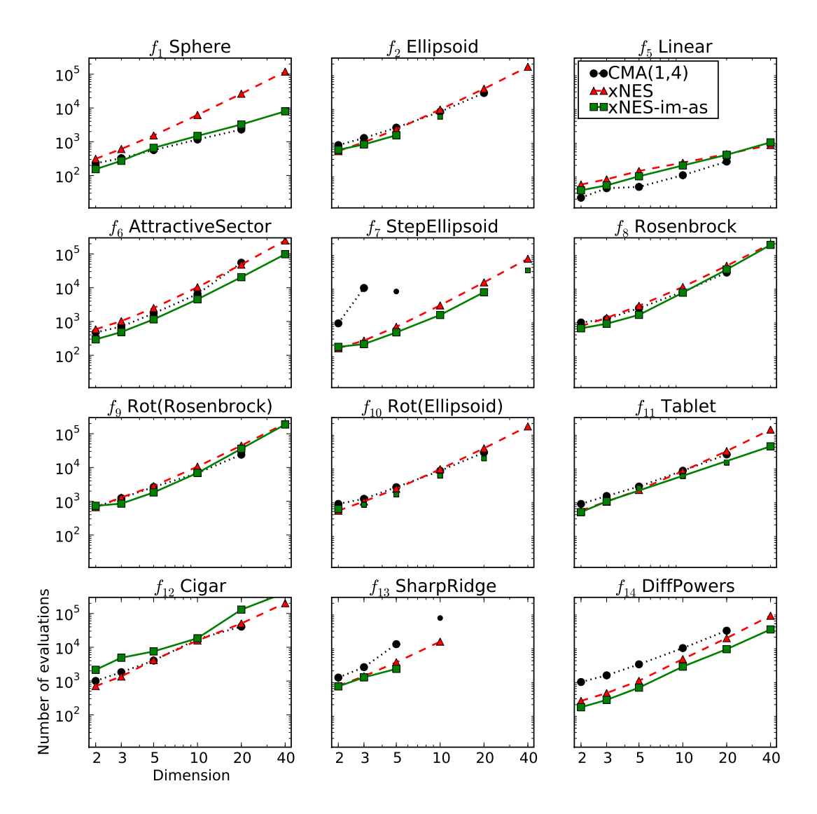
Figure 7: Unimodal benchmarks. Log-log plot of the median number of fitness evaluations (over 100 trials) required to reach the target fitness value of $-10^{-7}$ for the 12 unimodal benchmark functions on dimensions 2 to 40. Disconnected (smaller) plot markers denote cases where the corresponding algorithm converged prematurely in at least 50% of the runs (cases for which 90% or more prematurely converged are not shown at all). No data was available for (1,4)-CMA-ES on dimension 40. Note that xNES (red triangles) consistently solves all benchmarks, with a scaling factor that is almost the same over all functions. Also, xNES appears to be more stable, especially on the SharpRidge function. When employing importance mixing and adaptation sampling (xNES-im-as, green squares), performance increases, most substantially on the Sphere function, while robustness decreases.

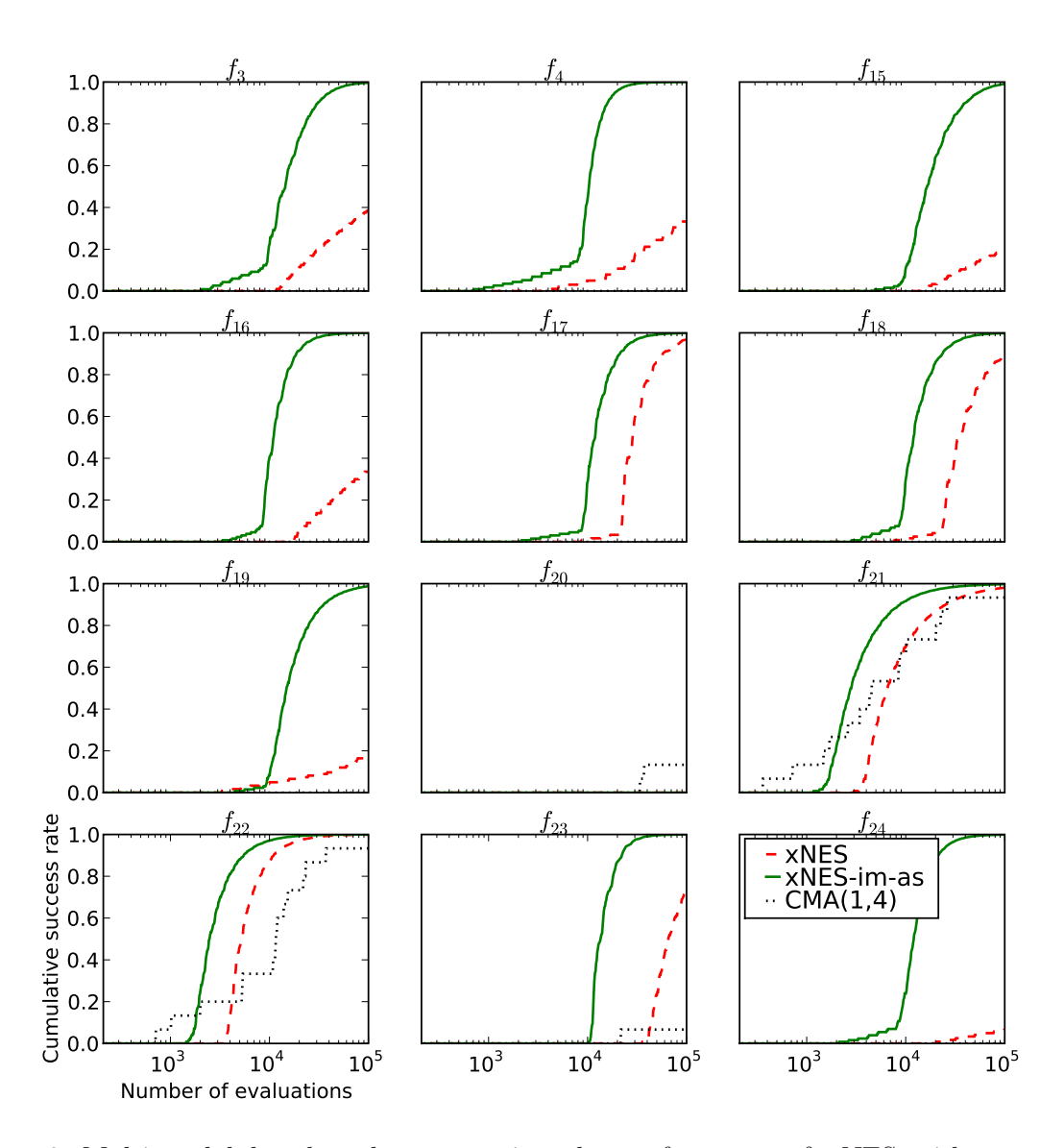
Figure 8: Multi-modal benchmarks, comparing the performance of xNES with restart strategies (dashed red) and (1,4)-CMA-ES (dotted black). Shown is the empirical cumulative success rate (over 100 runs, 15 for CMA-ES). Note that xNES clearly outperforms CMA-ES on all functions except $f_{21}$ and $f_{22}$ (both of which are simply combinations of 101 and 21 Gaussian peaks, respectively, without any global structure), where the results are very similar. When additionally employing importance mixing and adaptation sampling (xNES-im-as, solid green), performance improves even further.

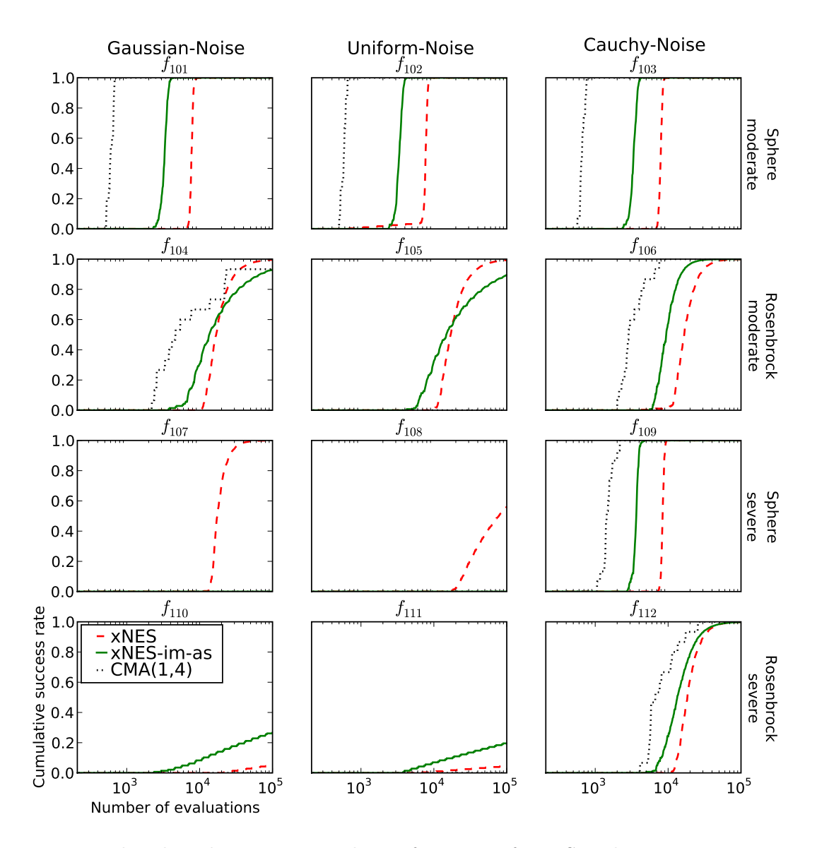
Figure 9: Noisy benchmarks, comparing the performance of xNES with restart strategies (dashed red), and (1,4)-CMA-ES (dotted black). Shown is the empirical cumulative success rate (over 100 runs, 15 for CMA-ES). The benchmarks are grouped by type of noise (vertical) and underlying function (horizontal). Generally speaking, Cauchy-noise is the least harmful, as the rare outliers do not affect the ranks all that much. We find that xNES outperforms CMA-ES on the majority of the functions. Additionally employing importance mixing and adaptation sampling (xNES-im-as, solid green), however, improves performance only on some of the functions. Continued in Figure 10.

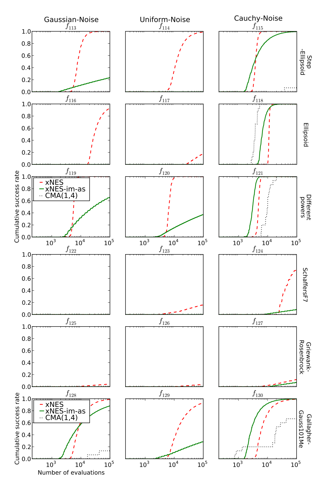
Figure 10: Noisy benchmarks (continued).

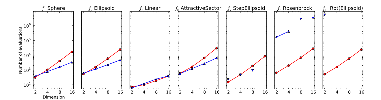
Figure 11: Comparison of the performance of xNES (red circles) and SNES (blue triangles) on a subset of the unimodal BBOB benchmark functions. The log-log plots show the median number of evaluations required to reach the target fitness $10^{-7}$ , for problem dimensions ranging from 2 to 16 (over 20 runs). The first 4 benchmark functions are separable, the other three are not. The inverted triangles indicate cases where SNES converged to the optimum in less than 90% of the runs.

understanding its behavior and in particular its limitations in more detail. Furthermore, the algorithm is specifically designed to scale gracefully to high-dimensional search problems. We thus apply SNES to two tasks with a scalable and considerably high search space dimension, namely neuro-evolutionary controller design, and the problem of finding low energy states in Lennard-Jones potentials.

6.3.1 Separable and Non-Separable Benchmarks

First, we evaluate SNES on a subset of the unimodal benchmark problems from the BBOB framework (Hansen and Finck, 2010a; Hansen and Auger, 2010). These benchmarks test the capability of SNES to descend quickly into local optima, a key property of most evolution strategies. The results in figure 11 show how SNES dominates when the function is separable ( $f_1$ through $f_6$ ), and converges much slower than xNES in non-separable benchmarks, as expected. In particular, on the rotated ellipsoid function $f_{10}$ , which is designed to make separable methods fail, SNES requires 4 orders of magnitude more evaluations. In dimensions d > 2 it fails completely because the resolution of double precision numbers is insufficient for this task.

6.3.2 Neuro-evolution

In the second experiment, we show how SNES is well-suited for neuroevolution problems because they tend to be high-dimensional, multi-modal, but with highly redundant global optima (there is not a unique set of weights that defines the optimal behavior). In particular, we run it on Non-Markovian double pole balancing, a task which involves balancing two differently sized poles hinged on a cart that moves on a finite track. The single control consists of the force F applied to the cart, and observations include the cart's position and the poles' angles, but no velocity information, which makes this task partially observable.

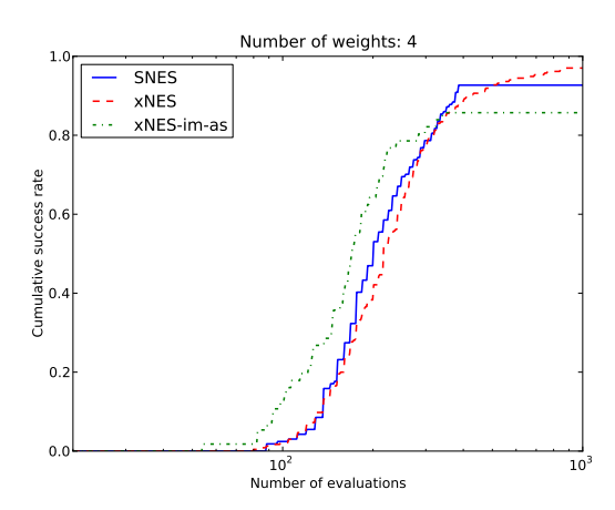
Figure 12: Left: Plotted are the cumulative success rates on the non-Markovian double-pole balancing task after a certain number of evaluations, empirically determined over 100 runs for each algorithm, using a single tanh-unit (n = 1) (i.e., optimizing 4 weights). We find that all three algorithm variants give state-of-the-art results, with a slightly faster but less robust performance for xNES with importance mixing and adaptation sampling. Right: Median number of evaluations required to solve the same task, but with increasing number of neurons (and corresponding number of weights). We limited the runtime to one hour per run, which explains why no results are available for xNES on higher dimensions (cubic time complexity). The fact that SNES quickly outperforms xNES, also in number of function evaluations, indicates that the benchmark is (sufficiently close to) separable, and it is unnecessary to use the full covariance matrix. For reference we also plot the corresponding results of the previously best performing algorithm CoSyNE (Gomez et al., 2008).

It provides a perfect testbed for algorithms focusing on learning fine control with memory in continuous state and action spaces (Wieland, 1991). The controller is represented by a simple recurrent neural network, with three inputs, (position x and the two poles' angles $\beta_1$ and $\beta_2$ ), and a variable number n of tanh units in the output layer, which are fully connected (recurrently), resulting in a total of n(n+3) weights to be optimized. The activation of the first of these recurrent neurons directly determines the force to be applied. We use the implementation found in PyBrain (Schaul et al., 2010).

An evaluation is considered a success if the poles do not fall over for 100,000 time steps. We experimented with recurrent layers of sizes n=1 to n=32 (corresponding to between 4 and 1120 weights). It turns out that a single recurrent neuron is sufficient to solve the task (Figure 12, left). In fact, both the xNES and SNES results are state-of-the-art, outperforming the previously best algorithm (CoSyNE; Gomez et al., 2008, with a median of 410 evaluations) by a factor two.

In practical scenarios however, we cannot know the best network size a priori, and thus the prudent choice consists in overestimating the required size. An algorithm that graciously scales with problem dimension is therefore highly desirable, and we find (Figure 12, right) that SNES is exhibiting precisely that behavior. The fact that SNES outperforms xNES with increasing dimension, also in number of function evaluations, indicates that the benchmark is separable, and it is unnecessary to use the full covariance matrix. We conjecture that this a property shared with the majority of neuroevolution problems that have enough weights to exhibit redundant global optima (some of which can be found without considering all parameter covariances).

6.3.3 Lennard-Jones Potentials

In our third benchmark, we show the performance of SNES on the widely studied problem of minimizing the Lennard-Jones atom cluster potentials, which is known for being extremely multi-modal (Wales and Doye, 1998). For that reason we employ the separable hill-climber variant (1+1)-SNES. The objective consists in finding that configuration of N atoms which minimizes the potential energy function

$$E_{LJ} \propto \sum_{i,j \le N} \left[ \left( \frac{1}{r_{ij}} \right)^{12} - \left( \frac{1}{r_{ij}} \right)^{6} \right] ,$$

where rij is the distance between atoms i and j (see also figure 13 for an illustration). For the setup here, we initialized µ near 0 and the step-sizes at σⁱ = 0.01 to avoid jumping into a local optimum in the fist generation. The results are plotted in figure 14, showing how SNES scales convincingly to hundreds of parameters (each run up to 500d function evaluations).

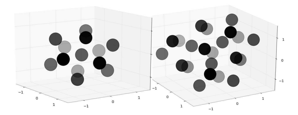
Figure 13: Illustration of the best configuration found for 13 atoms (symmetric, left), and 22 atoms (asymmetric, right).

6.4 Heavy Tails and Global Optimization

Can NES algorithms with heavy-tailed search distributions enhance the capability of escaping local optima? Our tests with the extremely heavy-tailed Cauchy distribution investigate the handling of multi-modality.

Figure 14: Performance of (1+1)-SNES on the Lennard-Jones benchmark for atom clusters ranging from 3 to 67 atoms (corresponding to problem dimensions d of 9 to 201). The yellow diamonds indicate the best known configurations (taken from (Wales and Doye, 1998)), and the box-plots show upper and lower quartile performance (the red line being the median) of SNES, over 100 runs. The inset is a zoom on the behavior in small dimensions, where SNES succeeds in locating the true optimum in a large fraction of the runs.

The first benchmark function is

$$f_{2Rosen}(\mathbf{z}) = \min \left\{ f_8(-\mathbf{z} - 10), 5 + f_8\left(\frac{\mathbf{z} - 10}{4}\right) \right\} ,$$

where f^{8} is the well-known Rosenbrock function (Hansen and Finck, 2010a), and the transformation (z−10)/4 is component-wise. Our variant has a deceptive double-funnel structure, with a large valley containing a local optimum and a smaller but deeper valley containing the global optimum. The global structure will tend to guide the search towards the local optimum (see also figure 15, left, for an illustration). For this experiment, the search distribution is initialized at mid-distance between the two optima, and the initial step-size σ is varied. Figure 15(right) shows the proportion of runs that converge to the global optimum, instead of the (easier to locate) local one, comparing for a multivariate Cauchy and Gaussian (1+1)-NES.

The second experiment uses the following 'random-basin' benchmark function:

$$f_{rb}(\mathbf{z}) = 1 - \frac{9}{10} r\left( \left\lfloor \frac{\mathbf{z}_1}{10} \right\rfloor, \dots, \left\lfloor \frac{\mathbf{z}_d}{10} \right\rfloor \right) - \frac{1}{10} r(\left\lfloor \mathbf{z}_1 \right\rfloor, \dots, \left\lfloor \mathbf{z}_d \right\rfloor) \cdot \prod_{i=1}^d \sin^2(\pi \mathbf{z}_i)^{\frac{1}{20d}}$$

to investigate the degree to which a heavy-tail distribution can be useful when the objective function is highly multi-modal, but there is no global structure to exploit. Here r : Z ^d ^→ [0, 1] is a pseudo-random number generator, which approximates an i.i.d. uniformly random distribution for each tuple of integers, while still being deterministic, i.e., each tuple evaluates to the same value each time. In practice, we implement it as a Mersenne twister (Matsumoto and Nishimura, 1998), seeded with the hash-value of the integers. Further, to avoid axis-alignment, we rotate the function by multiplying with an orthonormal random d × d matrix.

One interesting property of this function is that each unit-sized hypercube is an "attractor" of a local optimum. Thus, while sampling points from one hypercube, an ES will contract its search distribution, making it harder to escape from that local optimum. Furthermore, the values of the local optima are uniformly distributed in [0, 1], and do not provide a systematic global trend (in contrast to the Rastrigin function). If the optimization results in a value of, say, 0.11, then we know that only 11% of the local optima are better than this.

Figure 16 shows the results: not surprisingly, employing the Cauchy distribution for search permits longer jumps, and thus enables the algorithm to find better local optima on average. The Cauchy version outperforms the Gaussian version by a factor of two to three, depending on the problem dimension. Note that the improvement (for both distributions) is due the number of neighbor-cubes increasing exponentially with dimension, thus increasing the chance that a relatively small jump will reach a better local optimum. At the same time, the adaptation of the step size is slowed down by the dimension-dependency of the learning rate, which leaves the algorithm more time to explore before it eventually converges into one of the local optima.

6.5 Results Summary

Our results have a number of implications. First of all, the results on the BBOB benchmarks show that NES algorithms are competitive with the state-of-the-art across a wide variety of black-box optimization problems.

Beyond this very general statement, we have demonstrated advantages and limitations of specific variants, and as such established the generality and flexibility of the NES framework. Experiments with heavy-tailed and separable distributions demonstrate the viability of the approach on high-dimensional and complex, deceptively multi-modal domains. We obtained best reported results on the difficult task of training a neural controller for double polebalancing. This test, together with good results on the Lennard-Jones problem, show the feasibility of the algorithm for real-world search and optimization problems.

The multi-start strategy, although simple and non-adaptive in spirit, brings considerable improvements on many difficult multi-modal benchmarks. Its technique of interleaving multiple runs has advantages over truly sequential restart strategies, waiting for convergence before restarting.

In summary, our results demonstrate that it is indeed possible for an algorithm with a clean derivation from first principles to achieve state-of-the-art to best performance in the heuristics-dominated field of black-box optimization.

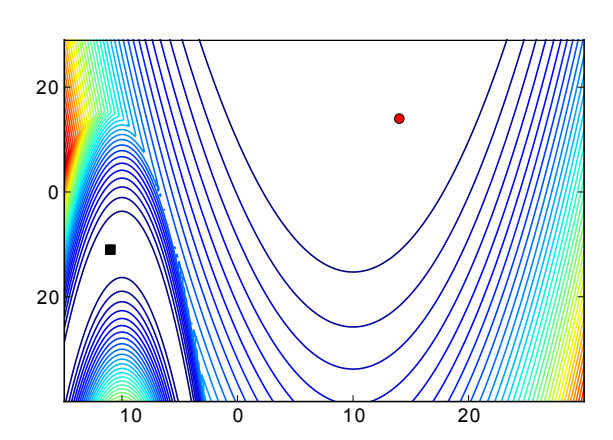
Figure 15: Left: Contour plot of the 2-dimensional Double-Rosenbrock function $f_{2Rosen}$ , illustrating its deceptive double-funnel structure. The global structure leads the search to the local optimum ((14,14), red circle), whereas the true optimum ((-11,-11), black square) is located in the smaller valley. Right: Empirical success probabilities (of locating the global optimum), evaluated over 200 runs, of 1000 function evaluations each, on the same benchmark, while varying the size of the initial search distribution. The results clearly show the robustness of using a heavy-tailed distribution.

7. Discussion

Technique	Issue addressed	Applicability	Relevant
		limited to	section
Natural gradient	Scale-invariance, many more	-	2.3
Fitness shaping	Robustness	-	3.1
Importance mixing	Performance, parameter sensitivity	-	3.2
Adaptation sampling	Performance, parameter sensitivity	-	3.3
Restart strategies	Reduced sensitivity to local optima	-	3.4
Exponential parameterization	Covariance constraints	Radial	4.1
Natural coordinate system	Efficiency	Radial	4.2

Table 2: Summary of enhancing techniques

Table 2 summarizes the various techniques we introduced. The plain search gradient suffers from premature convergence and lack of scale invariance (see section 2.2). Therefore, we use the natural gradient instead, which turns NES into a viable optimization method. To improve performance and robustness, we introduced several novel techniques. Fitness shaping makes the NES algorithm invariant to order-preserving transformations of the fitness function, thus increasing robustness. Importance mixing reduces the number of necessary samples to estimate the search gradient, while adaptation sampling adjusts NES's learn-

Figure 16: Left: Contour plot of (one instantiation of) the deceptive global optimization benchmark function $f_{rb}$ , in two dimensions. It is constructed to contain local optima in unit-cube-sized spaces, whose best value is uniformly random. In addition, it is superimposed on $10^d$ -sized regional plateaus, also with uniformly random value. Right: Value of the local optimum discovered on $f_{rb}$ (averaged over 250 runs, each with a budget of 100d function evaluations) as a function of problem dimension. Since the locally optimal values are uniformly distributed in [0,1], the results can equivalently be interpreted as the top percentile in which the found local optimum is located. E.g., on the 4-dimensional benchmark, NES with the Cauchy distribution tends to find one of the 6% best local optima, whereas employing the Gaussian distribution only leads to one of the best 22%.

ing rates online. Empirically we found that using both importance mixing and adaptation sampling yields highly performant results on the standard benchmarks. In addition, restart strategies substantially improve success probabilities on multi-modal functions and noisy benchmarks, clearly outperforming alternative approaches. Last, the exponential parameterization is crucial for maintaining positive-definite covariance matrices, and the use of the natural coordinate system guarantees computational feasibility.

NES applies to general parameterizable distributions. In this paper, we have experimentally investigated three variants, adjusted to the particular properties of different problem classes. We demonstrated the power of the xNES variant using a full multinormal distribution, which is invariant under arbitrary translations and rotations, on the canonical suite of standard benchmarks. Additionally, we showed that the restriction of the covariance matrix to a diagonal parameterization (SNES) allows for scaling to very high dimensions, both on the difficult non-Markovian double pole balancing task and the Lennard-Jones cluster potential optimization problem. Furthermore, we demonstrated that using heavy-tailed distributions (Cauchy) instead of Gaussian distributions yields substantial benefits in global optimization scenarios with multiple or deceptive local optima.

Unlike many black-box optimization algorithms, NES boasts a clean derivation from first principles. The relationship of NES to methods from other fields, notably evolution strategies (Hansen and Ostermeier, 2001) and policy gradients (Peters and Schaal, 2008; Kakade, 2002; Bagnell and Schneider, 2003), should be evident to readers familiar with both of these domains, as it marries the concept of fitness-based black-box optimization from evolutionary methods with the concept of Monte Carlo-based gradient estimation from the policy gradient framework.

7.1 Future Work

One intriguing possibility of extending NES starts by realizing that NES is not limited to continuous (flat) domains. In fact, NES can be designed to directly operate on discrete search spaces (e.g., graphs) or distributions with deep structure, such as deep belief networks and deep Boltzmann machines (Hinton and Salakhutdinov, 2006; Salakhutdinov and Hinton, 2009). This would allow us to find more complex solutions by combining and recombining building blocks produced by a deep network, opening up an interesting connection to genetic algorithms and their cross-over operators.

Program space constitutes one discrete search space of particular interest, and it seems promising to extend the NES approach to program search (genetic programming, Koza, 1992), building upon probabilistic representations of program trees (e.g., Salustowicz and Schmidhuber, 1997; Bosman and Jong, 2004) for which the natural gradient can be estimated.

Another possible direction of future research could comprise the investigation of sparsely parametrized distributions by means of which we can exploit selected covariance structure while keeping linear complexity, even in high dimensions. This structure can be either given in the problem domain (e.g., grouping weights by neuron (Gomez et al., 2008)) or learned incrementally.

Lastly, the approach is not necessarily restricted to purely following the gradient on expected fitness; for example, the objective could be formulated differently, as in including a trade-off between fitness and information gain (Schmidhuber, 2009).

7.2 Conclusion

In this paper, we introduced Natural Evolution Strategies, a novel family of algorithms that constitutes a principled alternative to standard stochastic search methods such as evolutionary algorithms. Maintaining a parameterized distribution on the set of solution candidates, the natural gradient is used to update the distribution's parameters in the direction of higher expected fitness.

A collection of techniques have been introduced, which addresses issues of convergence, robustness, computational complexity, sensitivity to hyperparameters, and sampling methods for algorithm speed. We investigated a number of instantiations of the NES family, ranging from general-purpose multi-variate normal distributions to heavy-tailed and separable distributions specialized in global optimization and high dimensionality, respectively. The results show best published performance on various standard benchmarks, as well as competitive performance on others.

In conclusion, NES algorithms are high-performing, derived from first principles and easy to implement. Their clean conceptual framework allows for a broad range of intriguing future developments.

Acknowledgments

This research was funded through the 7th framework program of the European Union, under grant number 231576 (STIFF project), SNF grants 200020-116674/1, 200021-111968/1 and 200020-122124/1, and SSN grant Sinergia CRSIK0-122697. We thank Faustino Gomez for helpful suggestions and his CoSyNE data, as well as Jan Peters, Nikolaus Hansen and Andreas Krause for insightful discussions.

Appendix A: Weighted Mann-Whitney Test

This appendix defines a Weighted Mann-Whitney test, as used in section 3.3 for virtual adaptation sampling. Although the derivations are trivial, the authors are not aware of any previous attempt to create a test with the same purpose.

Background. The classical Mann-Whitney test determines (with confidence $\rho$ ) whether two sets of samples $S = \{s_i\}$ and $S' = \{s_i'\}$ are likely to come from the same distribution. For that, the so-called U-statistic is computed:

$$U = \sum_{s_i > s_i'} 1 + \sum_{s_i = s_i'} \frac{1}{2}$$

Let $\mu = \frac{nn'}{2}$ and $\sigma = \sqrt{\frac{nn'(n+n'+1)}{12}}$ , where n and n' are the number of samples in S and S', respectively. We can then determine the significance of the difference between S and S'. They are different with confidence $\rho$ if:

$\Phi(\frac{U-\mu}{\sigma}) > 1 \rho$ (if S has larger values), or
$\Phi(\frac{U-\mu}{\sigma}) < \rho$ (if S' has larger values).

Introducing Weights. Now, assume that every sample in S and S' has a (positive) weight $(w_i \text{ or } w_i')$ associated to it. We can generalize the Mann-Whitney test by interpreting the weights as fractional number of occurrences in the sets:

$$U = \sum_{s_i > s'_j} w_i w'_j + \sum_{s_i = s'_j} \frac{1}{2} w_i w'_j$$

Accordingly, we also need to adjust the number of samples: $m = \sum_{i=1}^n w_i$ and $m' = \sum_{i=1}^{n'} w_i'$ , and thus $\mu = \frac{mm'}{2}$ and $\sigma = \sqrt{\frac{mm'(m+m'+1)}{12}}$ . We can see this weighted U-statistic as an interpolation between the cases covered

We can see this weighted U-statistic as an interpolation between the cases covered classical one. In fact, if the weights are integers, a sample s with weight w can be replaced equivalently by w occurrences of the same sample s (each with weight 1).

References

Y. Akimoto, Y. Nagata, I. Ono, and S. Kobayashi. Bidirectional Relation between CMA Evolution Strategies and Natural Evolution Strategies. In Parallel Problem Solving from Nature (PPSN), 2010.
S. Amari. Natural gradient works efficiently in learning. Neural Computation, 10(2):251– 276, 1998.
S. Amari and S. C. Douglas. Why natural gradient? In Proceedings of the 1998 IEEE International Conference on Acoustics, Speech, and Signal Processing (ICASSP '98), volume 2, pages 1213–1216, 1998.
A. Auger. Convergence results for the (1,λ)-SA-ES using the theory of φ-irreducible Markov chains. Theoretical Computer Science, 334(1-3):35 – 69, 2005.
J. A. Bagnell and J. Schneider. Covariant policy search. In Proceedings of the 18th international joint conference on Artificial intelligence, pages 1019–1024, San Francisco, CA, USA, 2003. Morgan Kaufmann Publishers Inc.
H.-G. Beyer. The theory of evolution strategies. Springer-Verlag New York, Inc., New York, NY, USA, 2001. ISBN 3-540-67297-4.
H.-G. Beyer and H.-P. Schwefel. Evolution strategies: A comprehensive introduction. Natural Computing, 1:3–52, 2002. ISSN 1567-7818.
P. A. Bosman and E. D. D. Jong. Learning Probabilistic Tree Grammars for Genetic Programming. In Parallel Problem Solving from Nature - PPSN VIII, volume 3242 of Lecture Notes in Computer Science, pages 192–201, Berlin, Heidelberg, 2004. Springer Berlin Heidelberg.
E. Cartan. Sur la repr´esentation g´eom´etrique des syst`e ´ mes mat´erieles non holonomes. In Proc Int Congr Math, Bologna, volume 4, pages 253–261, 1928.
F. Friedrichs and C. Igel. Evolutionary tuning of multiple svm parameters. Neurocomputing, 64:107–117, 2005.
T. Glasmachers and C. Igel. Gradient-based Adaptation of General Gaussian Kernels. Neural Computation, 17(10):2099–2105, 2005.
T. Glasmachers, T. Schaul, and J. Schmidhuber. A Natural Evolution Strategy for Multi-Objective Optimization. In Parallel Problem Solving from Nature (PPSN), 2010a.
T. Glasmachers, T. Schaul, Y. Sun, D. Wierstra, and J. Schmidhuber. Exponential Natural Evolution Strategies. In Genetic and Evolutionary Computation Conference (GECCO), Portland, OR, 2010b.
D. E. Goldberg. Genetic Algorithms in Search, Optimization and Machine Learning. Addison-Wesley Longman Publishing Co., Inc., Boston, MA, USA, 1st edition, 1989. ISBN 0201157675.
F. Gomez, J. Schmidhuber, and R. Miikkulainen. Accelerated Neural Evolution through Cooperatively Coevolved Synapses. Journal of Machine Learning Research, 2008.
N. Hansen and A. Auger. Real-parameter black-box optimization benchmarking 2010: Experimental setup, 2010.
N. Hansen and S. Finck. Real-parameter black-box optimization benchmarking 2010: Noiseless functions definitions, 2010a.
N. Hansen and S. Finck. Real-Parameter Black-Box Optimization Benchmarking 2010: Noisy Functions Definitions, 2010b.
N. Hansen and A. Ostermeier. Completely derandomized self-adaptation in evolution strategies. Evolutionary Computation, 9(2):159–195, 2001.
N. Hansen, A. S. P. Niederberger, L. Guzzella, and P. Koumoutsakos. A method for handling uncertainty in evolutionary optimization with an application to feedback control of combustion. Trans. Evol. Comp, 13:180–197, 2009.
M. Hasenj¨ager, B. Sendhoff, T. Sonoda, and T. Arima. Three dimensional evolutionary aerodynamic design optimization with CMA-ES. In Proceedings of the 2005 conference on Genetic and evolutionary computation, GECCO '05, pages 2173–2180, New York, NY, USA, 2005. ACM.
G. Hinton and R. Salakhutdinov. Reducing the dimensionality of data with neural networks. Science, 313(5786):504 – 507, 2006.
J. H. Holland. Adaptation in natural and artificial systems. MIT Press, Cambridge, MA, USA, 1992. ISBN 0-262-58111-6.
C. Igel and M. Husken. Empirical evaluation of the improved rprop learning algorithm. Neurocomputing, 50:2003, 2003.
G. A. Jastrebski and D. V. Arnold. Improving Evolution Strategies through Active Covariance Matrix Adaptation. In IEEE Congress on Evolutionary Computation, 2006.
M. Jebalia, A. Auger, M. Schoenauer, F. James, and M. Postel. Identification of the isotherm function in chromatography using cma-es. In IEEE Congress on Evolutionary Computation, pages 4289–4296, 2007.
M. Jebalia, A. Auger, and N. Hansen. Log-linear convergence and divergence of the scaleinvariant (1+1)-ES in noisy environments. Algorithmica, pages 1–36, 2010. online first.
S. Kakade. A natural policy gradient. Advances in Neural Information Processing Systems 14, 2:1531–1538, 2002.
J. Kennedy and R. Eberhart. Swarm Intelligence. Morgan Kaufmann, San Francisco, CA, 2001.
S. Kirkpatrick, C. D. Gelatt, Jr, and M. P. Vecchi. Optimization by Simulated Annealing. Science, 220:671–680, 1983.
J. Klockgether and H. P. Schwefel. Two-phase nozzle and hollow core jet experiments. In Proc. 11th Symp. Engineering Aspects of Magnetohydrodynamics, pages 141–148, 1970.
J. R. Koza. Genetic Programming: On the Programming of Computers by Means of Natural Selection. Cambridge, MA, 1992.
S. Kullback and R. A. Leibler. On information and sufficiency. The Annals of Mathematical Statistics, 22(1):79–86, 1951. ISSN 00034851.
P. Larra˜naga. Estimation of Distribution Algorithms. A New Tool for Evolutionary Computation, chapter An introduction to probabilistic graphical models, pages 25–54. Kluwer Academic Publishers, 2002.
M. Matsumoto and T. Nishimura. Mersenne twister: a 623-dimensionally equidistributed uniform pseudo-random number generator. Acm Transactions On Modeling And Computer Simulation, 8(1):3–30, 1998. ISSN 10493301.
S. D. Muller, J. Marchetto, S. Airaghi, and P. Koumoutsakos. Optimization based on bacterial chemotaxis. IEEE Transactions on Evolutionary Computation, 6:6–16, 2002.
I. Najfeld and T. F. Havel. Derivaties of the Matrix Exponential and Their Computation. Adv. Appl. Math, 16:321–375, 1994.
J. A. Nelder and R. Mead. A Simplex Method for Function Minimization. The Computer Journal, 7(4):308–313, 1965.
J. Peters. Machine Learning of Motor Skills for Robotics. PhD thesis, epartment of Computer Science, University of Southern California, 2007.
J. Peters and S. Schaal. Natural actor-critic. Neurocomputing, 71(7-9):1180–1190, 2008. ISSN 0925-2312.
I. Rechenberg and M. Eigen. Evolutionsstrategie: Optimierung technischer Systeme nach Prinzipien der biologischen Evolution. Frommann-Holzboog Stuttgart, 1973.
M. Riedmiller and H. Braun. A direct adaptive method for faster backpropagation learning: The RPROP algorithm. In IEEE International Conference on Neural Networks, pages 586–591. IEEE Press, 1993.
R. Ros and N. Hansen. A Simple Modification in CMA-ES Achieving Linear Time and Space Complexity. In R. et al., editor, Parallel Problem Solving from Nature, PPSN X, pages 296–305. Springer, 2008.
R. Y. Rubinstein and D. P. Kroese. The Cross-Entropy Method: A Unified Approach to Combinatorial Optimization, Monte-Carlo Simulation and Machine Learning (Information Science and Statistics). Springer, 2004.
R. Salakhutdinov and G. Hinton. Deep Boltzmann machines. In Proceedings of the International Conference on Artificial Intelligence and Statistics, volume 5, pages 448–455, 2009.
R. P. Salustowicz and J. Schmidhuber. Probabilistic Incremental Program Evolution. Evolutionary Computation, 5:123–141, 1997.
T. Schaul and J. Schmidhuber. Metalearning. Scholarpedia, 5(6):4650, 2010a.
T. Schaul and J. Schmidhuber. Towards Practical Universal Search. In Conference on Artificial General Intelligence (AGI), Lugano, 2010b.
T. Schaul, J. Bayer, D. Wierstra, Y. Sun, M. Felder, F. Sehnke, T. R¨uckstieß, and J. Schmidhuber. PyBrain. Journal of Machine Learning Research, 11:743–746, 2010.
T. Schaul, T. Glasmachers, and J. Schmidhuber. High Dimensions and Heavy Tails for Natural Evolution Strategies. In To appear in: Genetic and Evolutionary Computation Conference (GECCO), 2011.
J. Schmidhuber. Simple Algorithmic Theory of Subjective Beauty, Novelty, Surprise, Interestingness, Attention, Curiosity, Creativity, Art, Science, Music, Jokes. Journal of SICE, 48(1):21–32, 2009.
H.-P. Schwefel. Numerische Optimierung von Computer-Modellen mittels der Evolutionsstrategie, volume 26. Birkhaeuser, Basel/Stuttgart, 1977.
J. Shepherd, D. McDowell, and K. Jacob. Modeling morphology evolution and mechanical behavior during thermo-mechanical processing of semi-crystalline polymers. Journal of the Mechanics and Physics of Solids, 54(3):467 – 489, 2006.
O. M. Shir and T. B¨ack. The second harmonic generation case-study as a gateway for es to quantum control problems. In Proceedings of the 9th annual conference on Genetic and evolutionary computation, GECCO '07, pages 713–721, New York, NY, USA, 2007. ACM.
R. Storn and K. Price. Differential evolution - a simple and efficient heuristic for global optimization over continuous spaces. J. of Global Optimization, 11:341–359, December 1997. ISSN 0925-5001.
Y. Sun, D. Wierstra, T. Schaul, and J. Schmidhuber. Stochastic Search using the Natural Gradient. In International Conference on Machine Learning (ICML), 2009a.
Y. Sun, D. Wierstra, T. Schaul, and J. Schmidhuber. Efficient Natural Evolution Strategies. In Genetic and Evolutionary Computation Conference (GECCO), 2009b.
D. Wales and J. Doye. Global Optimization by Basin-Hopping and the Lowest Energy Structures of Lennard-Jones Clusters Containing up to 110 Atoms. The Journal of Physical Chemistry A, 101(28):8, 1998.
A. Wieland. Evolving Neural Network Controllers for Unstable Systems. In Proceedings of the International Joint Conference on Neural Networks (Seattle, WA), pages 667–673, 1991.
D. Wierstra, T. Schaul, J. Peters, and J. Schmidhuber. Natural Evolution Strategies. In Proceedings of the Congress on Evolutionary Computation (CEC08), Hongkong. IEEE Press, 2008.
S. Winter, B. Brendel, and C. Igel. Registration of bone structures in 3d ultrasound and ct data: Comparison of different optimization strategies. International Congress Series, 1281:242 – 247, 2005.